Assortativity Coefficient

The Assortativity Coefficient was proposed to analyze mixing patterns in networks, and was originally applied to networks of sexual contacts and marriage matching (Newman, 2003; Newman and Girvan, 2002). It quantifies the mixing in a network by evaluating the relative “weight” of the diagonal in the mixing matrix (Bojanowski, 2014).

If we define \(e_{ij}\) as the fraction of edges in a network that connect a vertex of type \(i\) to one of type \(j\), then the assortativity coefficient can be defined as:

\[ r = \dfrac{\sum_i e_{ii} - \sum_i a_i \cdot b_i}{1 - \sum_i a_i \cdot b_i} = \dfrac{\text{Tr}\textbf{e} - || \textbf{e}^2 ||}{1 - ||\textbf{e}^2||} \]

where \(\sum_j e_{ij} = a_i\), \(\sum_i e_{ij} = b_j\), \(\textbf{e}\) is the matrix whose elements are \(e_{ij}\), \(||\textbf{x}||\) indicates the sum of all elements in the matrix \(\textbf{x}\), and \(\text{Tr}\textbf{e}\) is the trace of the matrix \(\textbf{e}\).

from netseg import assortativity_coefficient
import igraph as ig 
import matplotlib.pyplot as plt 
import random 
import numpy as np 
import matplotlib.patches as mpatches

%config InlineBackend.figure_format = 'retina'

COLORS = [
    '#2C486F',
    '#436796',
    '#5E8FAE',
    '#80BDD6',
    '#B1DDE0',
    "#fdf8e7",
    '#F8E5B2',
    '#F3CF63',
    '#E9A64C',
    '#E3843B',
    '#DA584E'
 ]

COLORS_NDIV = [
    '#FBE3C2',
    '#F2C88F',
    '#ECB27D',
    '#E69C6B',
    '#D37750',
    '#B9563F',
    '#92351E'
]


def make_symmetric_sbm(p_in, p_out, n_groups, nodes_per_group, membership, **kwargs):
    pref_matrix = [
        [p_in if i == j else p_out for j in range(n_groups)] 
        for i in range(n_groups)
    ]
    block_sizes = [nodes_per_group] * n_groups
    g = ig.Graph.SBM(pref_matrix, block_sizes, **kwargs)
    
    g.vs['membership'] = membership
    
    return g 

Basic Usage

You can calculate the assortativity coefficient with the assortativity_coefficient function in netseg.

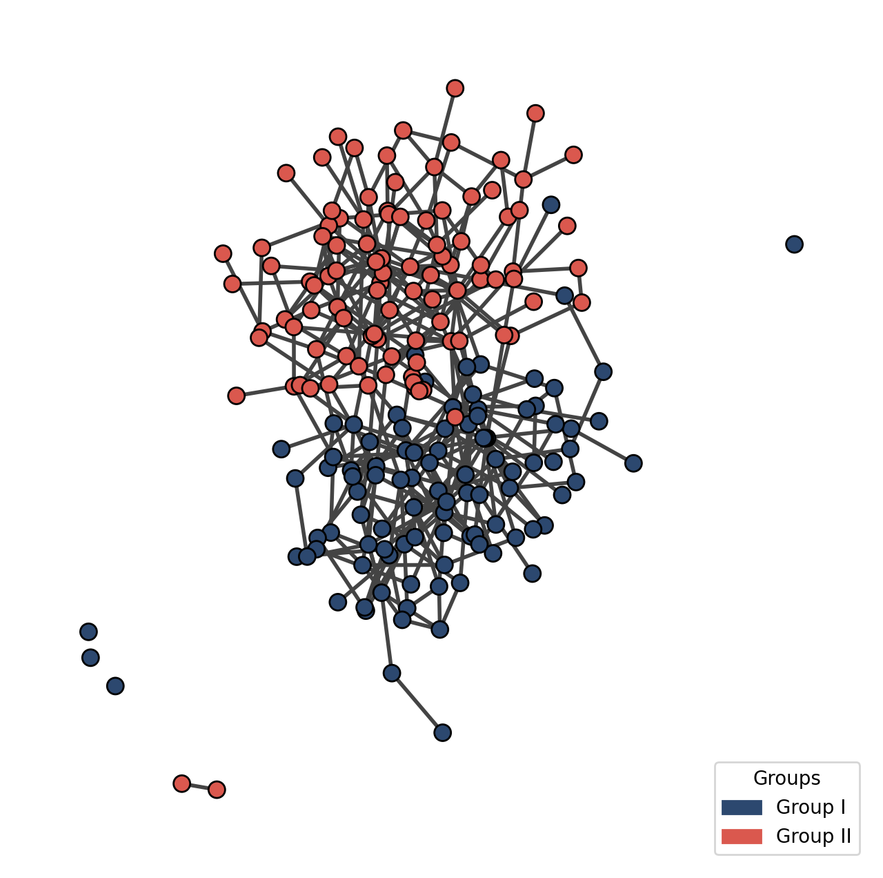
membership = [0 if i < 100 else 1 for i in range(200)]
g_simple = make_symmetric_sbm(0.03, 0.003, 2, 100,membership=membership)

fig, ax = plt.subplots(figsize = (8,8))
ig.plot(g_simple,
        vertex_size = 24, 
        vertex_color = [COLORS[0] if i == 0 else COLORS[-1] for i in g_simple.vs['membership']],
        layout = g_simple.layout_kamada_kawai(),
        target = ax)
g1_patch = mpatches.Patch(color=COLORS[0], label='Group I')
g2_patch = mpatches.Patch(color=COLORS[-1], label='Group II')
ax.legend(handles=[g1_patch, g2_patch], loc='lower right', title="Groups")
plt.show()

assort_coef = assortativity_coefficient("membership",g_simple)
print(assort_coef)

0.8479737535234044

Multiple Groups

random.seed(2)
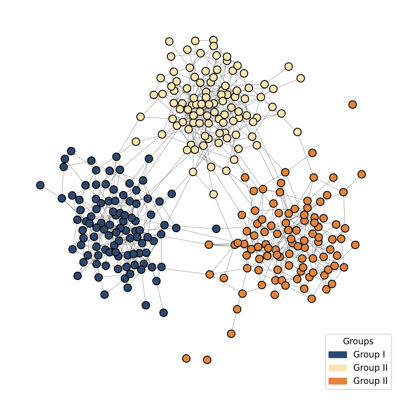
membership_multiple = ["foo"] * 100 + ["bar"] * 100 + ["baz"] * 100
colors_dict = {"foo":0, "bar":6, "baz":9}

fig, ax = plt.subplots(figsize = (8,8))
g_multiple = make_symmetric_sbm(0.04, 0.001, 3, 100, membership_multiple)

ig.plot(g_multiple, 
        vertex_size = 24,
        edge_arrow_size = 10.5, 
        edge_width = .3, 
        edge_color = "gray33",
        layout = g_multiple.layout_fruchterman_reingold(), 
        vertex_color = [COLORS[colors_dict[i]] for i in membership_multiple],
        target = ax)

g1_patch = mpatches.Patch(color=COLORS[0], label='Group I')
g2_patch = mpatches.Patch(color=COLORS[6], label='Group II')
g3_patch = mpatches.Patch(color=COLORS[9], label='Group II')
ax.legend(handles=[g1_patch, g2_patch,g3_patch], loc='lower right', title="Groups")
plt.show()

assort_coef_m = assortativity_coefficient("membership", g_multiple)
print(assort_coef_m)

0.9452061448782563

Example

We use the “AMEN Study (Catania)” dataset to demonstrate the Assortativity. Rather than individual node-by-node connections, this dataset provides a group-level mixing matrix of heterosexual partnerships between men (rows) and women (columns) in San Francisco neighborhoods. We measure the segregation with the demographic attribute “ethnicity”, divided into four categories: Black, Hispanic, White, and Other.

amen_catania_matrix = np.array([
    [506,  32,  26,  69],
    [ 23, 308,  38, 114],
    [ 10,  14,  32,  47],
    [ 26,  46,  68, 599]
])
assort_coef = assortativity_coefficient(membership= [], mixing_matrix= amen_catania_matrix)

# Since some measures require density, to evaluate the disconnected nodes netseg always expects a membership list. Nonetheless for the case of assortativity coefficient, since the calculation does not require density, an empty membership list can be passed.



print(assort_coef)

0.6214458753989227

References

• Bojanowski, M., & Corten, R. (2014). Measuring segregation in social networks. Social networks, 39, 14-32.

• Catania JA, Coates TJ, Kegeles S, Fullilove MT, Peterson J, Marin B, Siegel D, Hulley S. Condom use in multi-ethnic neighborhoods of San Francisco: the population-based AMEN (AIDS in Multi-Ethnic Neighborhoods) Study. Am J Public Health. 1992 Feb;82(2):284-7. doi: 10.2105/ajph.82.2.284. Erratum in: Am J Public Health 1992 Jul;82(7):998. PMID: 1739167; PMCID: PMC1694283.

• Newman, M.E.J., 2003. Mixing patterns in networks. Phys. Rev. A 67 (2), 1050–2947.

• Newman, M.E.J., Girvan, M., 2002. Mixing Patterns and Community Structure in Networks, arXiv:cond-mat/0210146 v1.