Segregation Matrix Index¶

Proposed by Fershtman (1997), Segregation Matrix Index (SMI) is designed to quantify the segregation in directed graphs based on the mixing matrix. Although the original measure assumes two groups, it is relatively easy to extend the measure for multiple groups (Bojanowski, 2014).

For each group, extended and normalized metric can be written as,

\[\frac{\pi_{internal} - \pi_{external}}{\pi_{internal} + \pi_{external}}\]

where \(\pi_{internal (external)}\) represents the internal (external) edge density. There is no specific reason to not to apply the metric for undirected networks except the proposed context dependent issues. Hence netseg allows metric to be used on undirected networks also, leaving the context to the end-user.

from netseg import smi
import igraph as ig 
import matplotlib.pyplot as plt 
from matplotlib.colors import LinearSegmentedColormap, to_hex, Normalize, BoundaryNorm
import random 
import numpy as np 
from time import perf_counter
from mpl_toolkits.axes_grid1 import make_axes_locatable
from matplotlib.cm import ScalarMappable
import matplotlib.patches as mpatches

%config InlineBackend.figure_format = 'retina'

COLORS = [
    '#2C486F',
    '#436796',
    '#5E8FAE',
    '#80BDD6',
    '#B1DDE0',
    "#fdf8e7",
    '#F8E5B2',
    '#F3CF63',
    '#E9A64C',
    '#E3843B',
    '#DA584E'
 ]

def make_symmetric_sbm(p_in, p_out, n_groups, nodes_per_group, membership, **kwargs):
    pref_matrix = [
        [p_in if i == j else p_out for j in range(n_groups)] 
        for i in range(n_groups)
    ]
    block_sizes = [nodes_per_group] * n_groups
    g = ig.Graph.SBM(pref_matrix, block_sizes, **kwargs)
    
    g.vs['membership'] = membership
    
    return g 

Basic Usage¶

membership= [0 if i < 200 else 1 for i in range(400)]
random.seed(3)
g = make_symmetric_sbm(0.04, 0.004, 2, 200,membership, directed = True)
fig,ax = plt.subplots(figsize = (8,8))

ig.plot(g, 
        vertex_size = 24,
        edge_color = "black",
        vertex_color = [COLORS[2] if i == 0 else COLORS[-3] for i in membership],
        edge_width = 0.3,
        edge_arrow_size = .6,
        layout = g.layout_kamada_kawai(),
        target = ax)

g1 = mpatches.Patch(color = COLORS[2], label = "Group I")
g2 = mpatches.Patch(color = COLORS[-3], label = "Group II")

ax.legend(handles = [g1,g2], loc = "lower right", title = "Nodal Attributes")
plt.show()

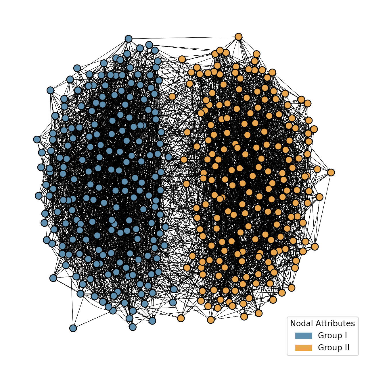
_images/0fcdd5880546ca8945876792fba7b3cbe62891a5f92aeb88946f54cf69a5a1ee.png

smi_scores = smi("membership", g)
print(smi_scores)

[0.80485054 0.82119777]

It is possible to find network level SMI if aggregated=True.

smi_network_level = smi("membership", g, aggregated= True)
print(smi_network_level)

0.8130241551452938

Multiple Groups¶

membership_multiple = ["foo"] * 200 + ["bar"] * 200 + ["baz"] * 200

colors_dict = {"foo":3, "bar":9, "baz":6}
random.seed(4)
g_multiple = make_symmetric_sbm(0.08, 0.001, 3, 200, membership_multiple, directed = True)
fig, ax = plt.subplots(figsize = (8,8))
ig.plot(g_multiple, vertex_size = 24, edge_arrow_size = .6, edge_width = .3, layout = g_multiple.layout_kamada_kawai(), vertex_color = [COLORS[colors_dict[i]] for i in membership_multiple], target = ax)
g1 = mpatches.Patch(color = COLORS[3], label = "Group I")
g2 = mpatches.Patch(color = COLORS[6], label = "Group II")
g3 = mpatches.Patch(color = COLORS[9], label = "Group II")

ax.legend(handles = [g1,g2,g3], loc = "lower right", title = "Nodal Attributes")
plt.show()

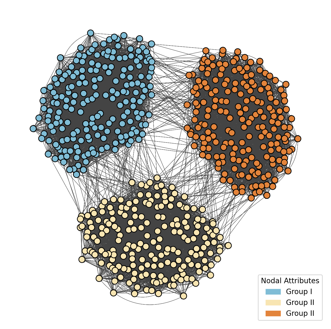
_images/edaa87e88cdef851f181e9d3be20f560e45c32cf2f29b4f85b76f2df70e18f21.png

smi_multiple = smi("membership", g_multiple, aggregated= False)
print(smi_multiple)

[0.94610731 0.95403488 0.94896782]

Example¶

We use the “Italian Gangs” dataset to demonstrate the SMI. Edges indicate co-membership in a gang. We measure the segregation with the nodal attribute “country of origin”. In the resulting plot, colors represent the different countries of origin. Original dataset can be found here.

g_example = ig.Graph.Read_GML('../assets/italian_gangs/italian_gangs.gml')
fig, ax = plt.subplots(figsize = (8,8))
random.seed(2)
ig.plot(g_example,
        layout = g_example.layout_kamada_kawai(),
        vertex_color = [COLORS[int(i)] for i in g_example.vs['country']],
        target = ax,
        edge_width = 0.4)
plt.show()

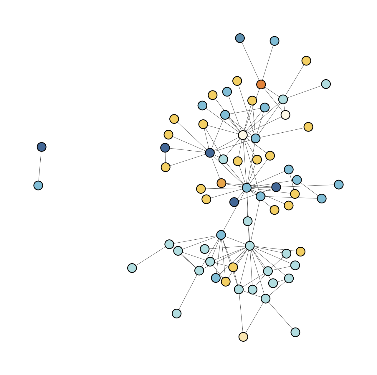
_images/267a580496957ec5181350fc92782ca76bc74275bb7f551bcc7744ffc83dc7e9.png

smi_score_example = smi("country", g_example, loops = False)

UserWarning: smi is defined for **directed** networks. Supplied graph at 0x1204abf40 is directed. Although it is extended for undirected networks in netseg, this extension is not the original definition of the authors.
UserWarning: Some group attributes only exist in a single node.
 If loops argument is False, this would result with NAs.
 If loops argument is True, network densities are calculated with self-loops allowed.
Read the docs at: https://onurb.codeberg.page/netseg/smi.html
/Users/onurtuncaybal/miniconda3/envs/netseg/lib/python3.14/site-packages/netseg/netseg.py:619: RuntimeWarning: invalid value encountered in divide
  densities = mixing_matrix / clique_matrix

Notice the warnings above. There are two UserWarning’s. Firstly, if you are applying a metric that is defined for an undirected (directed) network by its original authors to a directed (undirected) network, netseg will raise a warning.

But most importantly, the second UserWarning indicates that some membership values only exists in one node. Due to calculation of density, this immediately raises a warning. If you set loops = True, this warning can be avoided, that decision is context dependent, whether the network allows self loops should be decided by the user.

If you are using this metric on an aggregated level, singular memberships will cause average calculation to return NA. As can be seen below,

smi_score_example = smi("country", g_example, loops = False, aggregated= True)

UserWarning: smi is defined for **directed** networks. Supplied graph at 0x1204abf40 is directed. Although it is extended for undirected networks in netseg, this extension is not the original definition of the authors.

print(smi_score_example)

nan

If your network contextually allows it, you can add self loops for density calculations. This would return the aggregated value, but be mindful that it would skew the value to -1.

smi_score_example = smi("country", g_example, loops = True, aggregated= True)

UserWarning: smi is defined for **directed** networks. Supplied graph at 0x1204abf40 is directed. Although it is extended for undirected networks in netseg, this extension is not the original definition of the authors.
UserWarning: Some group attributes only exist in a single node.
 If loops argument is False, this would result with NAs.
 If loops argument is True, network densities are calculated with self-loops allowed.
Read the docs at: https://onurb.codeberg.page/netseg/smi.html

print(smi_score_example)

-0.8026732939947503

The above score indicates integration. Nonetheless, if we use the metric on the group level we can see that integregation is much less.

smi_score_example = smi("country", g_example, loops = True, aggregated= False)
print(smi_score_example)

[-0.60632689 -1.         -0.69565217 -0.40875497 -0.51332561 -1.
 -1.         -1.         -1.        ]

UserWarning: smi is defined for **directed** networks. Supplied graph at 0x1204abf40 is directed. Although it is extended for undirected networks in netseg, this extension is not the original definition of the authors.
UserWarning: Some group attributes only exist in a single node.
 If loops argument is False, this would result with NAs.
 If loops argument is True, network densities are calculated with self-loops allowed.
Read the docs at: https://onurb.codeberg.page/netseg/smi.html

References¶

Bojanowski, M., & Corten, R. (2014). Measuring segregation in social networks. Social networks, 39, 14-32.
Fershtman, M., 1997. Cohesive group segregation detection in a social network by the Segregation Matrix Index. Soc. Netw. 19, 193–207.