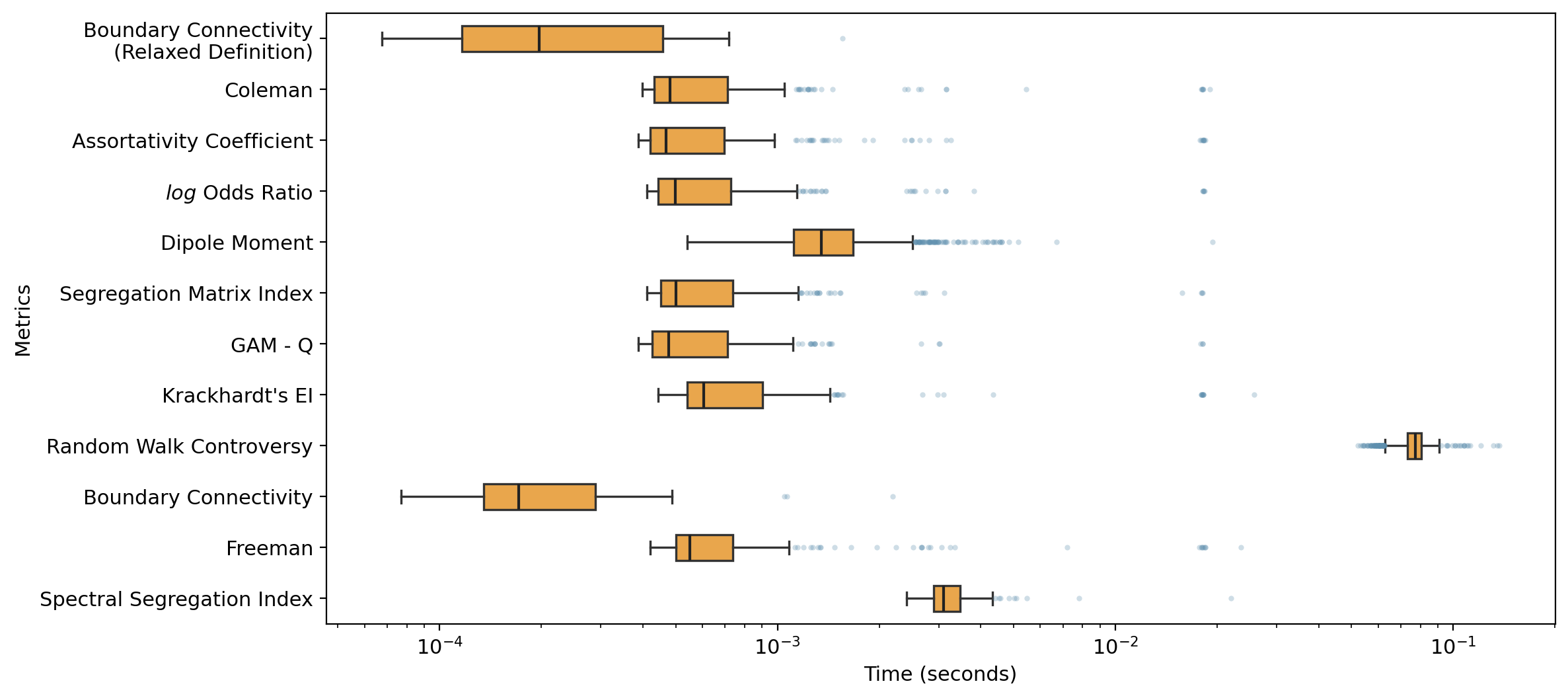
Behaviour
This section investigates the behavior of the metrics within the context of basic generative statistical model.
import matplotlib.pyplot as plt
import scipy.stats as stats
from matplotlib.colors import LinearSegmentedColormap, Normalize
from matplotlib.colors import to_hex
import igraph as ig
from matplotlib.patches import FancyArrow
import numpy as np
import contextlib
from time import perf_counter
from netseg import *
import warnings
from itertools import product
%config InlineBackend.figure_format = 'retina'
plt.rcParams.update({'font.size': 11, 'font.family': 'sans-serif'})

COLORS = [
    '#2C486F',
    '#436796',
    '#5E8FAE',
    '#80BDD6',
    '#B1DDE0',
    "#fdf8e7",
    '#F8E5B2',
    '#F3CF63',
    '#E9A64C',
    '#E3843B',
    '#DA584E'
 ]

COLORS_NDIV = [
    '#FBE3C2',
    '#F2C88F',
    '#ECB27D',
    '#E69C6B',
    '#D37750',
    '#B9563F',
    '#92351E'
]

cmap_custom = LinearSegmentedColormap.from_list("custom_gradient", COLORS)
cmap_ndiv =  LinearSegmentedColormap.from_list("custom_gradient", COLORS_NDIV)

def get_custom_colors_hex(values):
    vmin = min(values)
    vmax = max(values)

    norm = Normalize(vmin=vmin, vmax=vmax)
    custom_cmap = LinearSegmentedColormap.from_list("custom_gradient", COLORS)

    return [to_hex(custom_cmap(i)) for i in norm(values)]


def gaussian_mixture_model(mu_1, mu_2, sigma_1, sigma_2, n_1, n_2):
    """
    Create samples from a Gaussian mixture model with normalization to [-1,1].

    Parameters:
    -----------
    mu_1, mu_2: float
        Means of the two Gaussian components
    sigma_1, sigma_2: float
        Standard deviations of the two Gaussian components
    n_1, n_2: int
        Number of samples to draw from each component

    Returns:
    --------
    samples: ndarray
        Combined samples from both distributions normalized to [-1,1]
    mixing_weights: tuple
        The mixing weights (π₁, π₂)
    """

    total_samples = n_1 + n_2
    mixing_weight_1 = n_1 / total_samples
    mixing_weight_2 = n_2 / total_samples

    samples_1 = np.random.normal(mu_1, sigma_1, size=n_1)
    samples_2 = np.random.normal(mu_2, sigma_2, size=n_2)


    all_samples = np.concatenate((samples_1, samples_2))

    min_val = np.min(all_samples)
    max_val = np.max(all_samples)


    normalized_samples = (all_samples - min_val) / (max_val - min_val) * 2 - 1

    return normalized_samples, (mixing_weight_1, mixing_weight_2)

def bimodality_coefficient(data):
    """
    Calculate the bimodality coefficient for a distribution.
    BC > 0.555 indicates bimodality.

    Args:
        data: numpy array of data points

    Returns:
        bc: bimodality coefficient
        is_bimodal: boolean indicating if distribution is bimodal
    """
    n = len(data)


    skewness = stats.skew(data)
    kurtosis = stats.kurtosis(data)


    bc = (skewness**2 + 1) / (kurtosis + 3 * ((n-1)**2) / ((n-2)*(n-3)))


    is_bimodal = bc > 0.555

    return bc, is_bimodal

def generate_opinion_network(opinions, alpha, beta1, beta2):
    """
    Generates an igraph network based on a latent space logistic edge
    probability model.
    """

    opinions = np.asarray(opinions)
    n_nodes = len(opinions)
    diff_matrix = np.abs(opinions[:, None] - opinions[None, :])
    sum_matrix = opinions[:, None] + opinions[None, :]
    logit_matrix = alpha + beta1 * diff_matrix + beta2 * sum_matrix
    prob_matrix = 1 / (1 + np.exp(-logit_matrix))
    random_matrix = np.random.rand(n_nodes, n_nodes)
    edge_mask = random_matrix < prob_matrix
    i_indices, j_indices = np.where(np.triu(edge_mask, k=1))
    edges = list(zip(i_indices, j_indices))
    g = ig.Graph(n=n_nodes, directed=False)
    g.vs["opinion"] = opinions
    g.vs['group_membership'] = [0 if i < len(opinions) // 2 else 1 for i in range(len(opinions))]
    g.add_edges(edges)


    return g
A Basic Generative Model
To showcase the behaviour of the metrics we are using a simple generative model that depends on the opinions of the agents. We first define an opinion space as a vector where each element represents an individual agent’s opinion on a single issue within a population. To generate individual opinions, we employ a Gaussian mixture model, which allows us to control the level of polarization by varying the means and variances of the underlying distributions. Formally, we model the opinion space as a vector \(X \in \mathbb{R}^n\), where each of the \(n\) agents holds a stance value between -1 and 1 on the topic.
To simulate opinion diversity and polarization, we generate the values of \(X\) independently from a two-component Gaussian mixture with means \(\mu_1\), \(\mu_2\) and standard deviations \(\sigma_1\), \(\sigma_2\), respectively:
This provides fine-grained control over both the separation (via \(\mu_1\), \(\mu_2\)) and the spread (via \(\sigma_1\), \(\sigma_2\)) of opinions on the topic. Although the model is flexible for varying levels and asymmetries of polarization, we are setting \(|\mu_1| = |\mu_2|\) for simplicity. By tuning these parameters, we can simulate different levels and asymmetries of polarization.
After normalizing the distribution, we use the bimodality coefficient to quantify the extent of opinion polarization. The bimodality coefficient for a finite sample is a descriptive measure that captures the presence and strength of bimodality in a distribution and is defined as:
where \(m_3\) is the skewness of the distribution, \(m_4\) refers to its excess kurtosis, and \(n\) refers to the sample size. The values of the bimodality coefficient range between 0 and 1. Greater values (above 5/9) indicate a bimodal distribution.
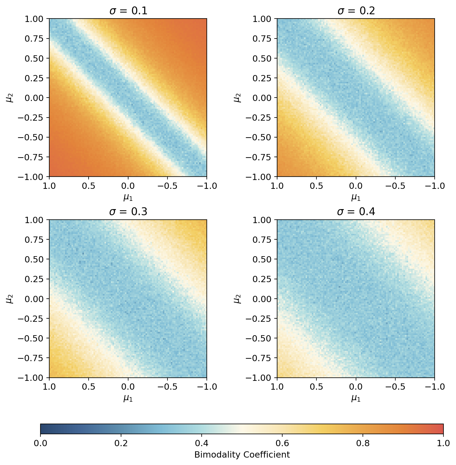
The influence of the parameters \(\mu_1, \mu_2, \sigma_1\), and \(\sigma_2\) on the opinion distribution as measured by the bimodality coefficient is illustrated in the figure below where we set \(\sigma_1 = \sigma_2\) for illustrative purposes. If we increase \(\sigma_1\) and \(\sigma_2\), the spread of each opinion cluster grows, resulting in lower bimodality coefficients. Meanwhile, \(\mu_1\) and \(\mu_2\) control the separation between the two modes, effectively determining the distance between ideological peaks. Together, these parameters shape the overall structure of the distribution and allow us to simulate varying levels of ideological polarization.
# For demonstration purposes we are setting the sigmas to equal values.
grid_size = 100
mu_values = np.linspace(-1, 1, grid_size)
sigmas = [0.1, 0.2, 0.3, 0.4]

fig, axes = plt.subplots(2, 2, figsize=(8, 8), layout = "constrained")
axes = axes.flatten()

for idx, sigma in enumerate(sigmas):
    bim_coef = np.empty((grid_size, grid_size))
    for i, m1 in enumerate(mu_values):
        for j, m2 in enumerate(mu_values):
            opinion_array, mm = gaussian_mixture_model(m1, m2, sigma, sigma, 200, 200)
            bc, __ = bimodality_coefficient(opinion_array)
            bim_coef[i, j] = bc

    ax = axes[idx]
    im = ax.imshow(bim_coef, extent=[1, -1, -1, 1], cmap=cmap_custom, vmin = 0, vmax = 1)

    ax.set_title(r'$\sigma$ = ' + f'{sigma}')
    ax.set_xlabel(r'$\mu_1$')
    ax.set_ylabel(r'$\mu_2$')

cbar = fig.colorbar(im, ax=axes, orientation='horizontal', shrink=0.95, aspect=40, label = "Bimodality Coefficient")
plt.show()
With the opinion space in place, we can start building the network itself. We parameterize our model with the following;
While \(\alpha\) will setup the overall density of the network, As \(\beta_1\) decreases (increases) nodes with higher difference will less (more) likely to connect. And according to the sign and value of the \(\beta_2\) there will be degree homogeneity within a certain group. Given this, we can demonstrate the networks as follows.
ALPHA = -2
BETA1S = [0, -2, -4]
BETA2S = [0, .3, .6]

params = list(product(BETA1S, BETA2S))
fig, axs = plt.subplots(3,3, figsize = (9,9))


opinion_array, __ = gaussian_mixture_model(0.5, -0.5, 0.2, 0.2, 100, 100)
graphs = []
for (b1,b2) in params:
  graphs.append(generate_opinion_network(opinion_array, ALPHA, b1, b2))
axs = axs.flatten()
for index, adj in enumerate(graphs):
  ig.plot(adj, vertex_size = 12, target = axs[index], edge_width = .2,
          vertex_color = get_custom_colors_hex(adj.vs['opinion']),
          layout = adj.layout_fruchterman_reingold())
  b1 = params[index][0]
  b2 = params[index][1]
  axs[index].set_title(rf"$\beta_1$ = {b1}, $\beta_2$ = {b2}", fontsize = 8)
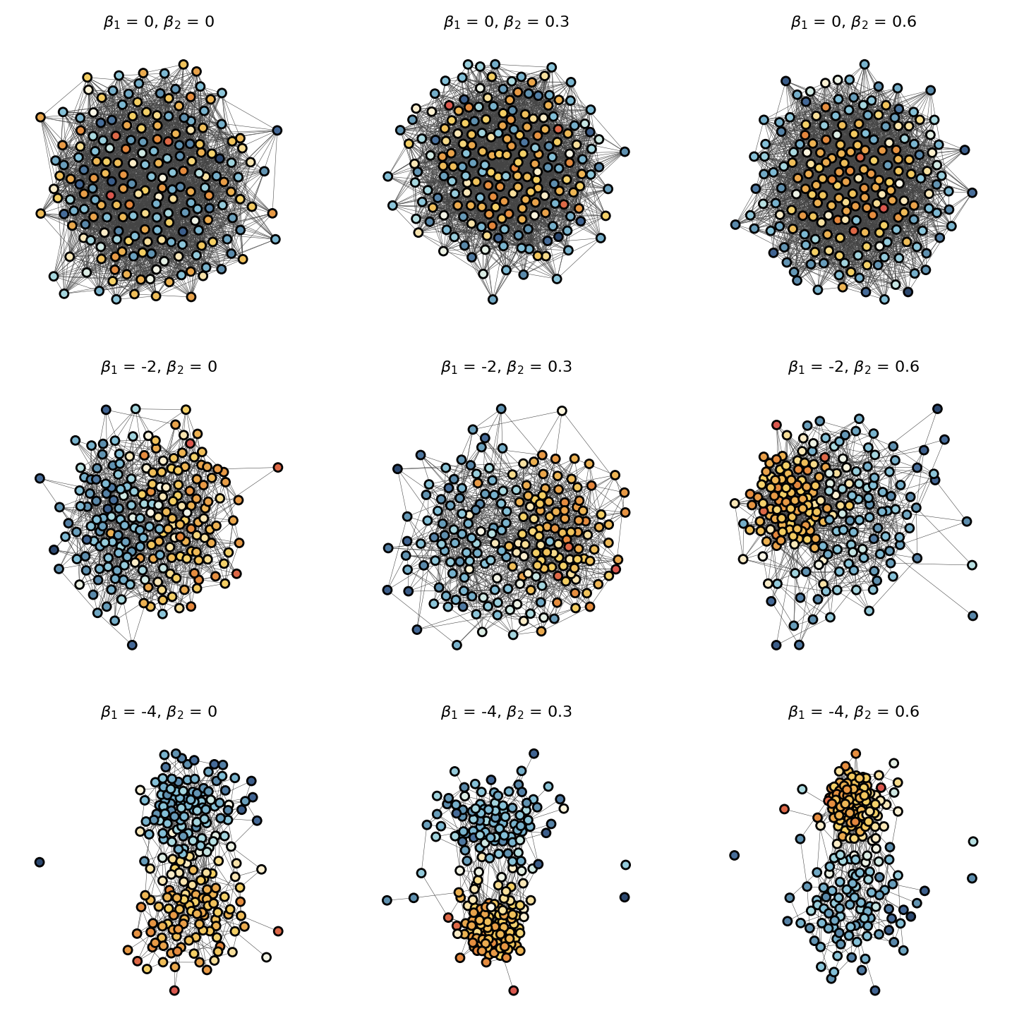
We can see generated example graphs above. Now we are generating a parameter space with higher resolution that is also demonstrating heterophily to demonstrate the behaviour of the metrics.
warnings.filterwarnings('ignore') # For passing an undirected network to a directed network measure.


@contextlib.contextmanager
def timer(times_dict, key):

    start_time = perf_counter()
    try:
        yield
    finally:
        end_time = perf_counter()
        times_dict[key] = end_time - start_time

def bm_netseg(network: ig.Graph, set_ops = False):
    _network = network.copy()
    if not set_ops:
        tot_vcount = network.vcount()
        _network.vs['membership'] = [0 if i < tot_vcount // 2 else 1 for i in range(tot_vcount)]
    else:
        _network.vs['opinion'] = [network.vs['opinion'][i] for i in network.vs['name']]
        _network.vs['membership'] = [0 if i < 0 else 1 for i in _network.vs['opinion']]


    scores = {}
    times = {}
    with timer(times, "ssi"):
        scores["ssi"] = ssi("membership", _network, aggregate=True)

    with timer(times, "freeman"):
        scores["freeman"] = freeman("membership", _network)

    with timer(times, "boundary"):
        scores["boundary"] = boundary_connectivity("membership", _network, relax=False)

    with timer(times, "rwc"):
        scores["rwc"] = random_walk_controversy("membership", _network, maximum_walk_length=1000, n_sim=1000, verbose=False, k_top=5, balanced=True)

    with timer(times, "ei"):
        scores["ei"] = krackhardt_ei("membership", _network)

    with timer(times, "gamq"):
        scores["gamq"] = gamix("membership", _network)

    with timer(times, "smi"):
        scores["smi"] = smi("membership", _network, aggregated=True)

    with timer(times, "dp"):
        scores["dp"] = dipole_moment("membership", _network, k_top=5, balanced=True)

    with timer(times, "orwg"):
        scores["orwg"] = orwg("membership", _network)

    with timer(times, "assort"):
        scores["assort"] = assortativity_coefficient("membership", _network)

    with timer(times, "coleman"):
        scores["coleman"] = coleman("membership", _network, network_level= True)

    with timer(times, "boundary_relaxed"):
        scores["boundary_relaxed"] = boundary_connectivity("membership", _network, relax = True)

    return {
        "scores": scores,
        "times": times
    }

metrics = [
    "ssi", "freeman", "boundary", "rwc", "ei",
    "gamq", "smi", "dp", "orwg", "assort", "coleman",
    "boundary_relaxed"
]

ALPHA = -2
BETA1S = [4, -4]
BETA2S = [0, .6]
RESOLUTION = 40

params = list(product(np.linspace(BETA1S[0],BETA1S[1], RESOLUTION), np.linspace(BETA2S[0],BETA2S[1], RESOLUTION)))
opinion_array, __ = gaussian_mixture_model(0.6, -0.6, 0.1, 0.1, RESOLUTION, RESOLUTION)
graphs = []


for index, (b1,b2) in enumerate(params):
  print(f'Generating Graphs || {index + 1} / {len(params)} OK!', end = "\r", flush= True)
  graphs.append(generate_opinion_network(opinion_array, ALPHA, b1, b2))
print("")

num_beta1 = len(BETA1S)
num_beta2 = len(BETA2S)
num_metrics = len(metrics)

scores = []
times = []
ecounts = []

for index, graph in enumerate(graphs):

    print(f'Benchmarking || {index + 1} / {len(graphs)} OK!', end = "\r", flush= True)
    results = bm_netseg(graph)
    scores.append(results['scores'])
    times.append(results['times'])
    ecounts.append(graph.ecount())
Generating Graphs || 1600 / 1600 OK!
Benchmarking || 1600 / 1600 OK!
fig, axs = plt.subplots(4, 3, figsize=(12, 16), layout="constrained")
axs = axs.flatten()

metrics_title = [
    "Spectral Segregation Index", "Freeman", "Boundary Connectivity", "Random Walk Controversy", "Krackhardt's EI",
    "GAM - Q", "Segregation Matrix Index", "Dipole Moment", r"$log$ Odds Ratio", "Assortativity Coefficient", "Coleman", "Boundary Connectivity\n(Relaxed Definition)"
]
metrics = [
    "ssi", "freeman", "boundary", "rwc", "ei",
    "gamq", "smi", "dp", "orwg", "assort", "coleman",
    "boundary_relaxed"
]

metric_bounds = {
    "ssi": (0, None),
    "freeman": (-1, 1),
    "boundary": (-0.5, 0.5),
    "rwc": (0, 1),
    "ei": (-1, 1),
    "gamq": (None, 1),
    "smi": (-1, 1),
    "dp": (0, 1),
    "orwg": (0, None),
    "assort": (None, 1),
    "coleman": (-1, 1),
    "boundary_relaxed": (-0.5, 0.5)
}

for index, metric in enumerate(metrics):
    score = [i[metric] for i in scores]
    score = np.array(score).reshape(RESOLUTION, RESOLUTION)

    vmin, vmax = metric_bounds[metric]

    im = axs[index].imshow(score,
                           cmap=cmap_custom,
                           extent=[0, .6, -4, 4],
                           aspect="auto",
                           vmin=vmin,
                           vmax=vmax)

    axs[index].set_ylabel(rf'$\beta_1$', fontsize=12)
    axs[index].set_xlabel(rf'$\beta_2$', fontsize=12)
    axs[index].set_title(metrics_title[index])
    fig.colorbar(im, ax=axs[index], orientation="horizontal", shrink=0.6)

plt.show()
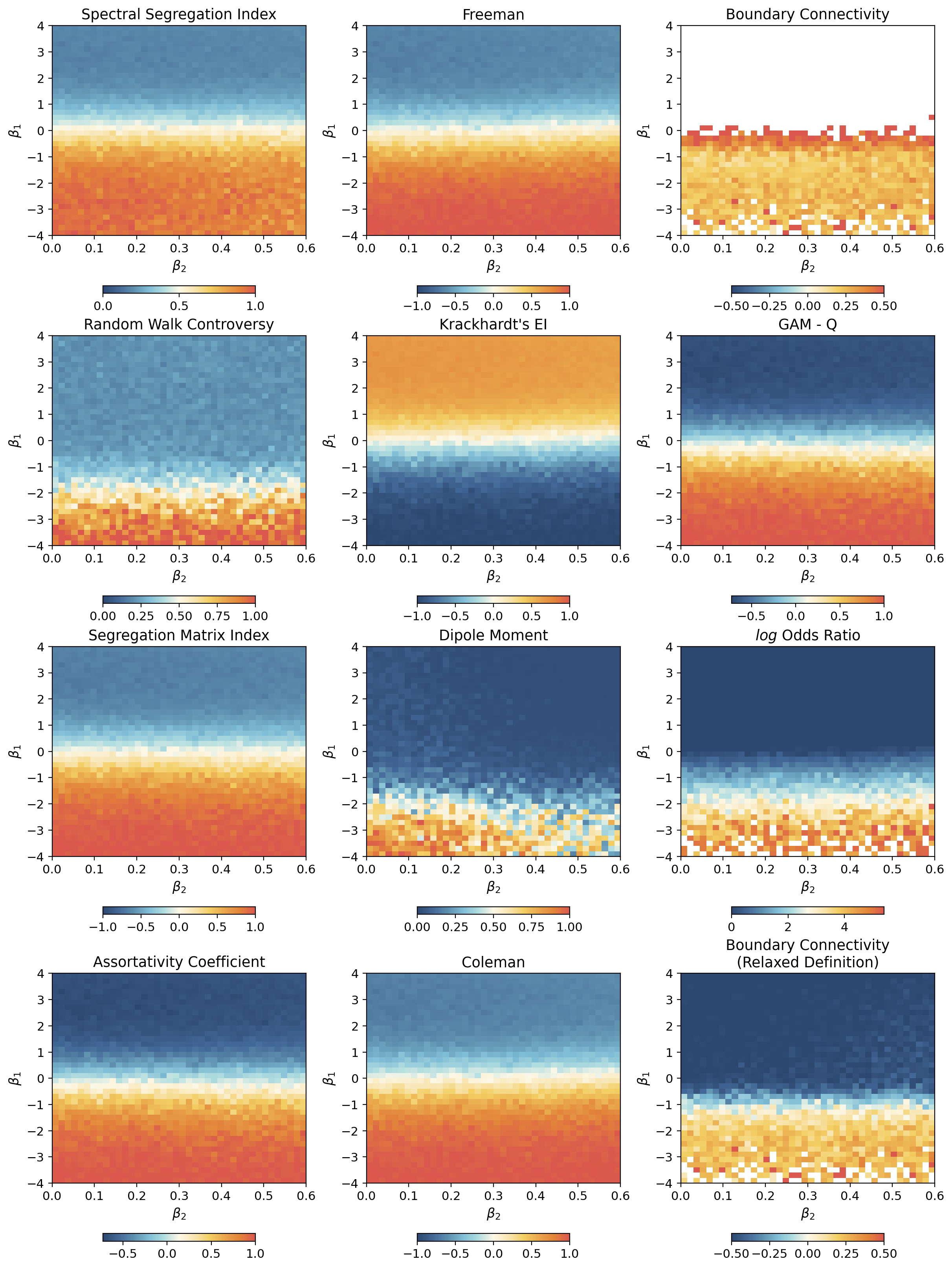
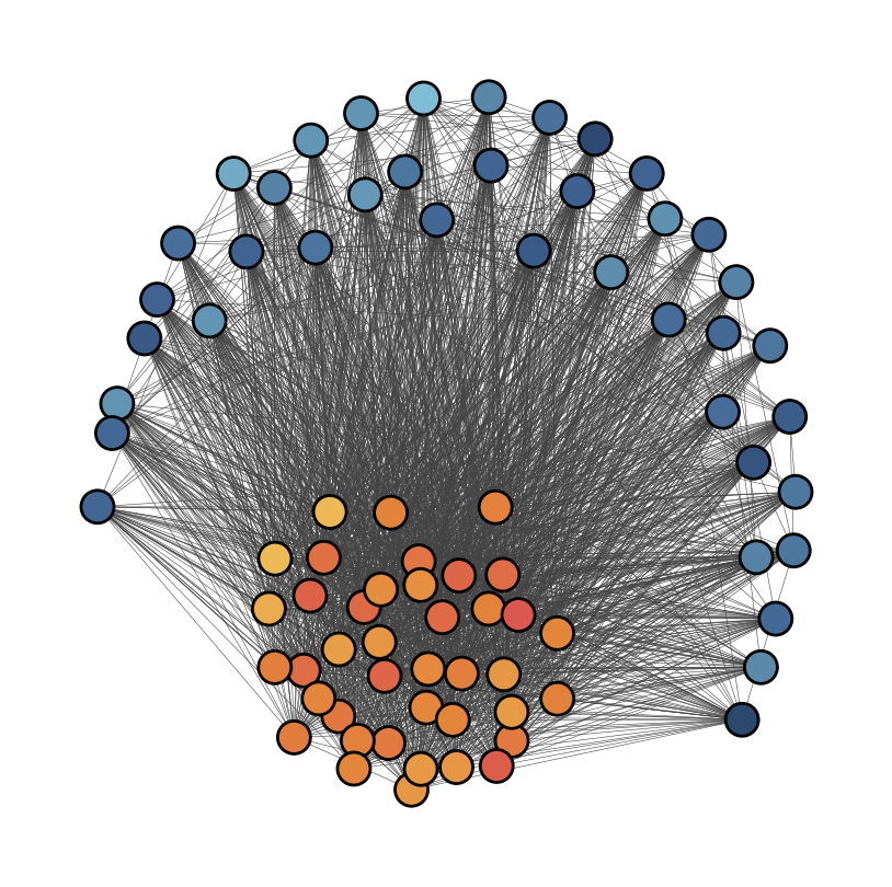
Occasionally, certain metrics fail to return a numeric value. This is expected behavior since the model sometimes generates networks that do not satisfy the logical prerequisites for these calculations. For example, for the below graph there are no boundary nodes, hence boundary connectivity can not be calculated.
fig, axs = plt.subplots(figsize = (5,5))
ig.plot(graphs[3],
        vertex_color = get_custom_colors_hex(graphs[-1].vs['opinion']),
        target = axs,
        layout = graphs[-1].layout_kamada_kawai(),
        edge_width = .2)
plt.show()
fig, axs2 = plt.subplots(figsize=(12, 6))

boxprops = dict(facecolor='#E9A64C', color='#333333', linewidth=1.2)
medianprops = dict(color='#222222', linewidth=1.5, solid_capstyle='butt')
whiskerprops = dict(color='#333333', linewidth=1.2)
capprops = dict(color= '#333333', linewidth=1.2)
flierprops = dict(marker='.', markerfacecolor='#5E8FAE', markersize=6,
                  markeredgecolor='none', alpha=0.3)


time_data = [[i[metric] for i in times] for metric in metrics]
axs2.boxplot(time_data, labels=metrics_title, vert=False, patch_artist= True, boxprops=boxprops, flierprops=flierprops, medianprops=medianprops, whiskerprops=whiskerprops, capprops=capprops)
axs2.set_xscale('log')
axs2.set_xlabel('Time (seconds)')
axs2.set_ylabel('Metrics')
plt.show()