Coleman’s Homophily Index

Coleman’s Homophily Index (Coleman, 1958) is a measure of segregation for directed networks. In the original formulation, the measure is defined for each subgroup of a population; nonetheless, netseg allows using the extended definition (Bojanowski, 2014) for the network level. The group-wise calculation can be given as:

\[\begin{split} S_{\text{Coleman}}^g = \begin{cases} \frac{m_{gg1} - m_{gg1}^*}{\sum_{i \in G_g} \eta_i - m_{gg1}^*} & \text{if} \quad m_{gg1} \geq m_{gg1}^*, \\[1.5em] \frac{m_{gg1} - m_{gg1}^*}{m_{gg1}^*} & \text{if} \quad m_{gg1} < m_{gg1}^* \end{cases} \end{split}\]

where \(m_{gg1}\) denotes the realized within-group ties in the \(g\)-th group, and \(m^*_{gg1}\) denotes the expected number of ties within the \(g\)-th group in a random network with the same edge density. This can be calculated as:

\[m^*_{gg1} = \sum_{i \in G_g} \eta_i \cdot \frac{n_g - 1}{N - 1}\]

where \(\eta_i\) is the out-degree of actor \(i\).

The metric ranges between \(-1\) (perfectly avoiding one’s own group) and \(1\) (perfect segregation). The index can easily be generalized for the network level with:

\[\omega^* = \sum_{g}\sum_{i \in G_g} \eta_i \frac{n_g - 1}{N - 1}\]

and then can be calculated with:

\[\begin{split}S_{\text{Coleman}} = \begin{cases} \frac{\omega - \omega^*}{\sum_{i=1}^N \eta_i - \omega^*} & \text{if} \quad \omega \geq \omega^*, \\[1.5em] \frac{\omega - \omega^*}{\omega^*} & \text{if} \quad \omega < \omega^*. \end{cases}\end{split}\]

from netseg import coleman
import igraph as ig 
import matplotlib.pyplot as plt 
from matplotlib.colors import LinearSegmentedColormap, to_hex, Normalize, BoundaryNorm
import random 
import numpy as np 
from time import perf_counter
from mpl_toolkits.axes_grid1 import make_axes_locatable
from matplotlib.cm import ScalarMappable
import matplotlib.patches as mpatches

%config InlineBackend.figure_format = 'retina'

COLORS = [
    '#2C486F',
    '#436796',
    '#5E8FAE',
    '#80BDD6',
    '#B1DDE0',
    "#fdf8e7",
    '#F8E5B2',
    '#F3CF63',
    '#E9A64C',
    '#E3843B',
    '#DA584E'
 ]

COLORS_NDIV = [
    '#FBE3C2',
    '#F2C88F',
    '#ECB27D',
    '#E69C6B',
    '#D37750',
    '#B9563F',
    '#92351E'
]

def make_symmetric_sbm(p_in, p_out, n_groups, nodes_per_group, membership, **kwargs):
    pref_matrix = [
        [p_in if i == j else p_out for j in range(n_groups)] 
        for i in range(n_groups)
    ]
    block_sizes = [nodes_per_group] * n_groups
    g = ig.Graph.SBM(pref_matrix, block_sizes, **kwargs)
    
    g.vs['membership'] = membership
    
    return g 

def get_custom_colors_hex(values):
    vmin = min(values)
    vmax = max(values)

    norm = Normalize(vmin=vmin, vmax=vmax)
    custom_cmap = LinearSegmentedColormap.from_list("custom_gradient", COLORS)
    
    return [to_hex(custom_cmap(i)) for i in norm(values)]

Basic Usage

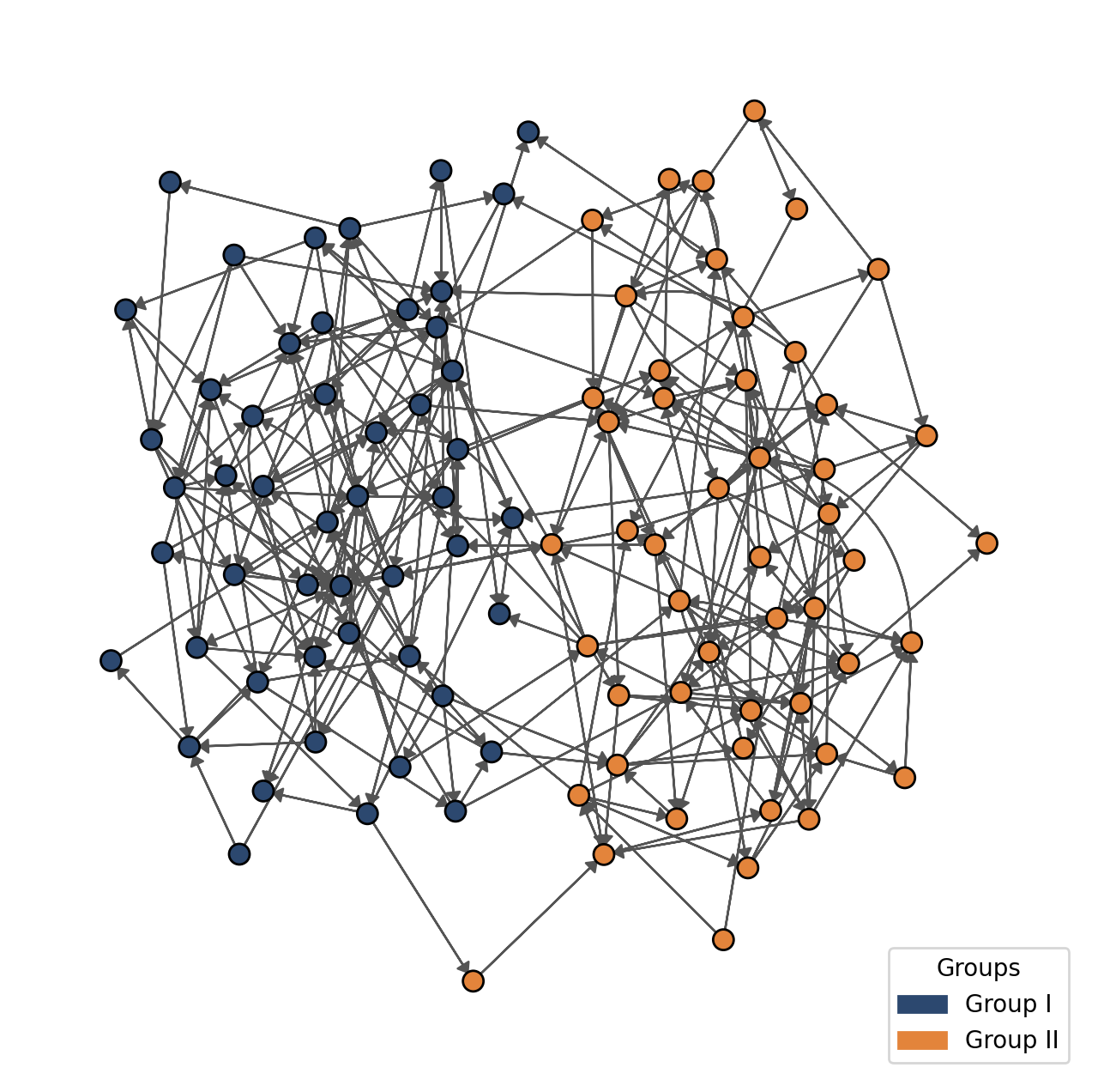
The most basic usage is the canonical definition that calculates the index for each group.

membership= [0 if i < 50 else 1 for i in range(100)]
random.seed(2)
g = make_symmetric_sbm(0.05, 0.004, 2, 50,membership, directed = True)

fig, ax = plt.subplots(figsize = (8,8))
ig.plot(g, 
        vertex_size = 24,
        edge_color = "gray33",
        vertex_color = [COLORS[0] if i == 0 else COLORS[9] for i in membership],
        edge_width = 0.9,
        edge_arrow_size = 10.5,
        layout = g.layout_kamada_kawai(),
        target = ax)
g1_patch = mpatches.Patch(color=COLORS[0], label='Group I')
g2_patch = mpatches.Patch(color=COLORS[9], label='Group II')
ax.legend(handles=[g1_patch, g2_patch], loc='lower right', title="Groups")
plt.show()

coleman_score = coleman(membership, g)
print(coleman_score)

[np.float64(0.8383673469387755), np.float64(0.8421739130434782)]

We can also calculate the score for the network level with setting the network_level parameter to True.

coleman_score_network_level = coleman(membership, g, network_level= True)
print(coleman_score_network_level)

0.8402105263157895

Multiple Groups

random.seed(2)
membership_multiple = ["foo"] * 100 + ["bar"] * 100 + ["baz"] * 100
colors_dict = {"foo":0, "bar":6, "baz":9}

fig, ax = plt.subplots(figsize = (8,8))
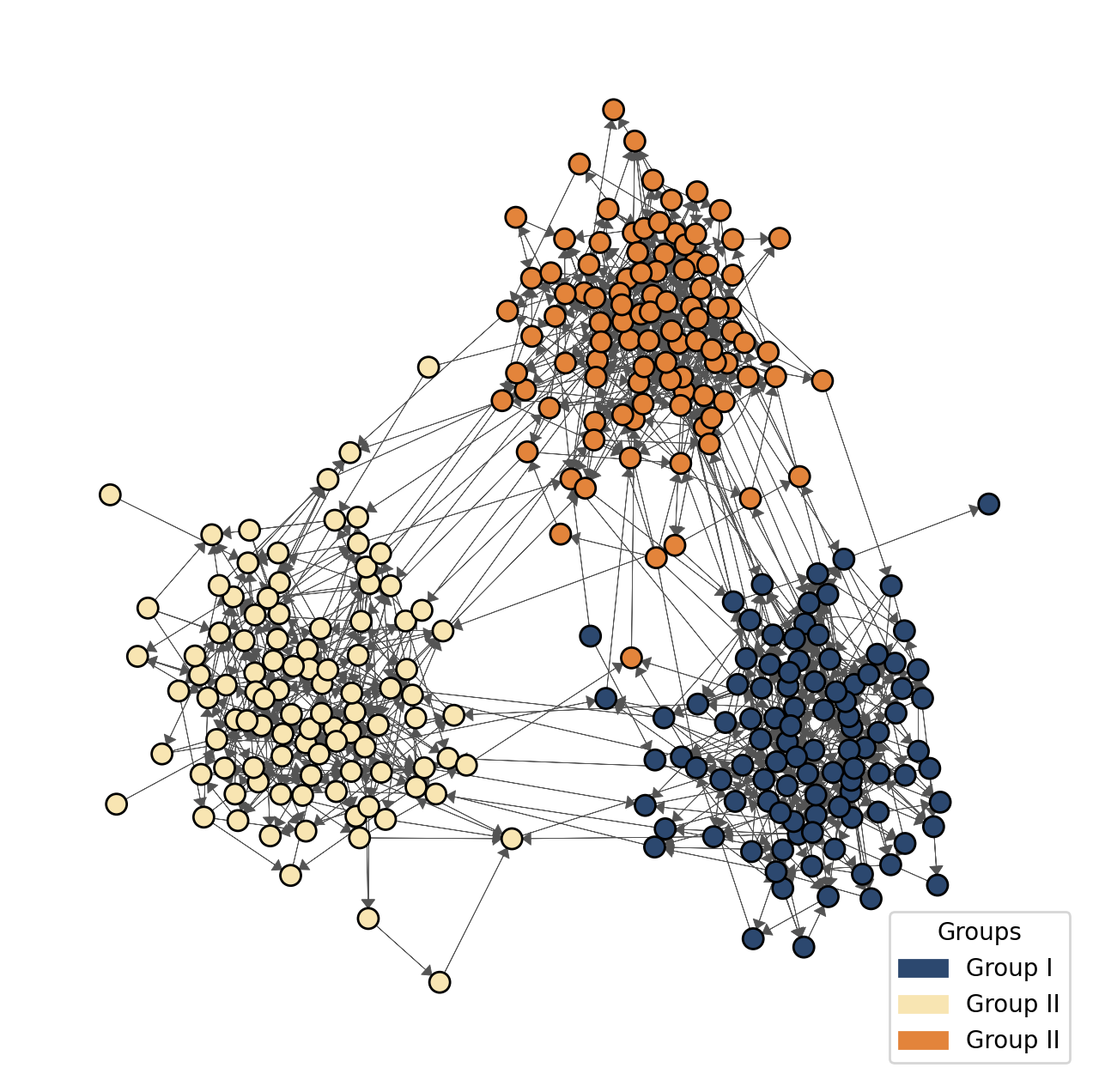
g_multiple = make_symmetric_sbm(0.03, 0.001, 3, 100, membership_multiple, directed = True)

ig.plot(g_multiple, 
        vertex_size = 24,
        edge_arrow_size = 10.5, 
        edge_width = .3, 
        edge_color = "gray33",
        layout = g_multiple.layout_fruchterman_reingold(), 
        vertex_color = [COLORS[colors_dict[i]] for i in membership_multiple],
        target = ax)

g1_patch = mpatches.Patch(color=COLORS[0], label='Group I')
g2_patch = mpatches.Patch(color=COLORS[6], label='Group II')
g3_patch = mpatches.Patch(color=COLORS[9], label='Group II')
ax.legend(handles=[g1_patch, g2_patch,g3_patch], loc='lower right', title="Groups")
plt.show()

coleman("membership", g_multiple) # Notice that g_multiple has the vertex_property 'membership'. 

[np.float64(0.9283546325878594),
 np.float64(0.8994957983193277),
 np.float64(0.9305727554179567)]

Notes on Null Model Selection

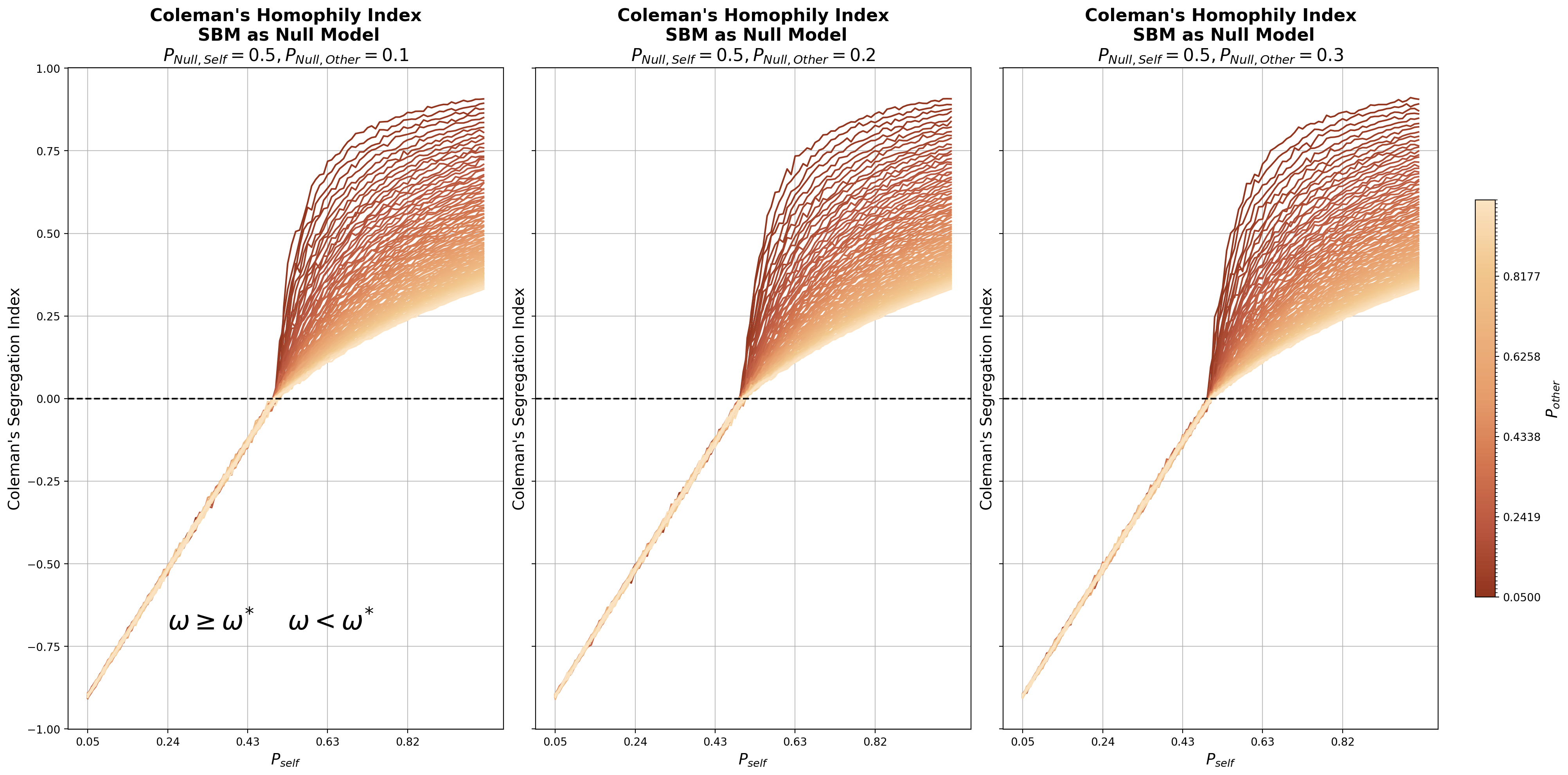
netseg allows custom null models. Nonetheless, especially in Coleman’s case, null model selection should be carefully evaluated since the metric itself is designed for the ER model only. Since Coleman’s Homophily Index is calculated differently according to the relationship between \(\omega\) and \(\omega^*\), only when \(\omega \geq \omega^*\) can an SBM act as a null model.

We can show the insensitivity to the outer edges of the SBM as the null model with the addition of the following code:

membership = [0 if i < 100 else 1 for i in range(200)]
g = make_symmetric_sbm(0.5, 0.1, 2, 100, membership, directed = True)
coleman_null_changing_self = [] 
for other in np.linspace(0.05, 1, 100):
    coleman_null_changing_self_sub = []
    for _self in np.linspace(0.05, 1, 100):
      null_models = [make_symmetric_sbm(_self, other, 2, 100, membership, directed = True) for i in range(20)]
      c = coleman(membership, g, None, null_models, True)
      coleman_null_changing_self_sub.append(c)
    
    coleman_null_changing_self.append(coleman_null_changing_self_sub)

coleman_changing_self = [] 
for other in np.linspace(0.05, 1, 100):
    coleman_changing_self_sub = []
    for _self in np.linspace(0.05, 1, 100):
      g = make_symmetric_sbm(_self, other, 2, 100, membership, directed = True)
      null_models = [make_symmetric_sbm(0.5, 0.1, 2, 100, membership, directed = True) for i in range(20)]
      c = coleman(membership, g, None, null_models, True)
      coleman_changing_self_sub.append(c)
    
    coleman_changing_self.append(coleman_changing_self_sub)

colemans_network_level_null_model_er = []

for other in np.linspace(0.01, 1, 100):
  colemans_network_level_sub = []
  for _self in np.linspace(0.01, 1, 100):  
    g = make_symmetric_sbm(_self, other, 2, 100, membership, directed = True)
    null_models = [ig.Graph.Erdos_Renyi(g.vcount(), g.density(), directed = True)]
    c = coleman(membership,g, None,null_models=null_models, network_level = True)
    colemans_network_level_sub.append(c)
  colemans_network_level_null_model_er.append(colemans_network_level_sub)

fig,axs = plt.subplots(1,3, figsize = (20 ,10), sharey=True)
cmap = LinearSegmentedColormap.from_list("custom_gradient", COLORS_NDIV[::-1])
_other = np.linspace(0.05, 1, 100)
bounds = _other
norm = BoundaryNorm(boundaries= bounds, ncolors = cmap.N)

for i, level in enumerate(coleman_null_changing_self):
  axs[0].plot(level, color = COLORS_NDIV[-1])

axs[0].grid(True, alpha = 0.8)
axs[0].set_xlabel(r'$P_{Null, self}$', fontsize = 14)
axs[0].set_ylabel(r"Coleman's Segregation Index", fontsize = 14)
sm = ScalarMappable(cmap = cmap, norm = norm)
sm.set_array([])


axs[0].set_title("Coleman's Homophily Index\n SBM as Null Model\n" + r"$P_{Self} = 0.5, P_{Other} = 0.1$", fontsize = 16, fontweight = "bold")
fig.tight_layout()
axs[0].set_xticks(range(len(_other))[::20])
axs[0].set_xticklabels([round(i,2) for i in np.linspace(0.05, 1, 100)[::20]])

for i, level in enumerate(coleman_changing_self):
  axs[1].plot(level, color = cmap(norm(_other[i])))

axs[1].grid(True, alpha = 0.8)
axs[1].set_xlabel(r'$P_{self}$', fontsize = 14)
axs[1].set_ylabel(r"Coleman's Segregation Index", fontsize = 14)
sm = ScalarMappable(cmap = cmap, norm = norm)
sm.set_array([])
axs[1].set_title("Coleman's Homophily Index\n SBM as Null Model\n" + r"$P_{Null,Self} = 0.5, P_{Null,Other} = 0.1$", fontsize = 16, fontweight = "bold")
fig.tight_layout()
axs[1].set_xticks(range(len(_other))[::20])
axs[1].set_xticklabels([round(i,2) for i in np.linspace(0.05, 1, 100)[::20]])
axs[1].axhline(0, linestyle = 'dashed', c = "black")


for i, level in enumerate(colemans_network_level_null_model_er):
  axs[2].plot(level, color = cmap(norm(_other[i])))

axs[2].grid(True, alpha = 0.8)
axs[2].set_xlabel(r'$P_{self}$', fontsize = 14)
axs[2].set_ylabel(r"Coleman's Segregation Index", fontsize = 14)
sm = ScalarMappable(cmap = cmap, norm = norm)
sm.set_array([])
cbar = fig.colorbar(sm, ax = axs, ticks = bounds[::20], fraction = 0.05, shrink = 0.6, pad = 0.025, orientation = "vertical")
cbar.set_label(r"$P_{other}$", size = 14, loc= "center")
cbar.ax.yaxis.set_label_position('right')
axs[2].set_title("Coleman's Homophily Index\n ER as Null Model\n", fontsize = 16, fontweight = "bold")
axs[2].set_xticks(range(len(_other))[::20])
axs[2].set_xticklabels([round(i,2) for i in np.linspace(0.05, 1, 100)[::20]])


axs[2].axhline(0, linestyle = 'dashed', c = "black")
axs[1].text(10, 0.15, r"$\omega \geq \omega^{*}$", fontsize = 24)
axs[1].text(10, -0.15, r"$\omega < \omega^{*}$", fontsize = 24)

axs[0].axvline(47, linestyle = 'dashed', c = "black")
axs[0].text(20, 0.-0.7, r"$\omega \geq \omega^{*}$",fontsize = 24)
axs[0].text(50, -0.7, r"$\omega < \omega^{*}$", fontsize = 24)
plt.show()

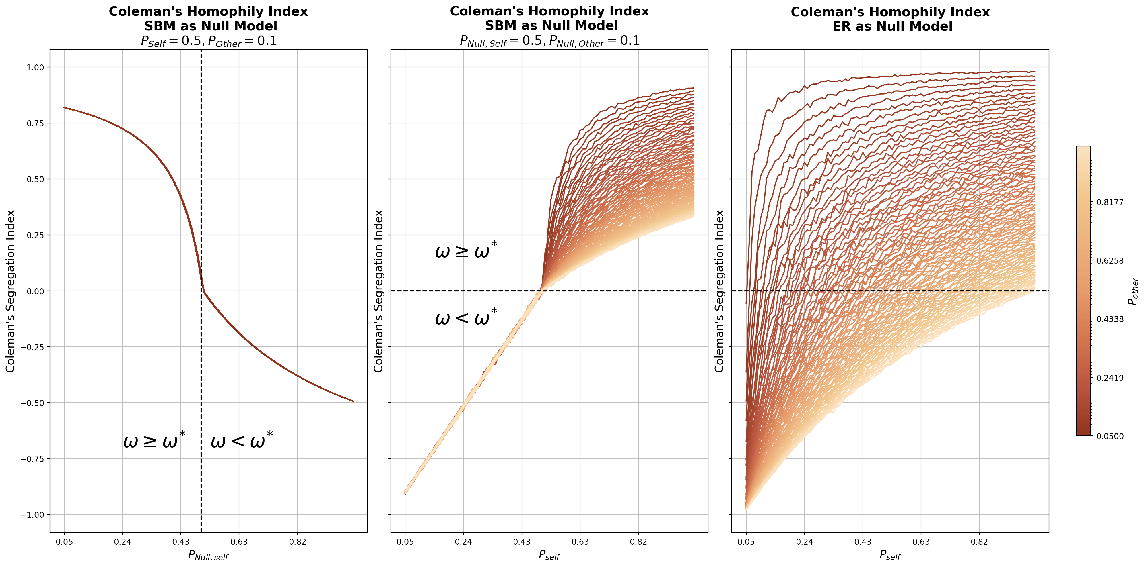
In the above plot, we are showing the change in the generative model where the null network is generated with \(P_{\text{Null,Self}} = 0.5\) and \(P_{\text{Null,Other}} = 0.1\). Coleman’s Index calculates as 0 when the realized number of edges within the group is equal to the number of edges within the group in the null model. This corresponds to the \(P_{\text{self}} = 0.5\) threshold. Before that, since the metric does not include the null model’s cross-group edges, altering the cross-group edges does not change the score.

coleman_changing_self_1 = [] 
for other in np.linspace(0.05, 1, 100):
    coleman_changing_self_sub = []
    for _self in np.linspace(0.05, 1, 100):
      g = make_symmetric_sbm(_self, other, 2, 100, membership, directed = True)
      null_models = [make_symmetric_sbm(0.5, 0.2, 2, 100, membership, directed = True) for i in range(20)]
      c = coleman(membership, g, None, null_models, True)
      coleman_changing_self_sub.append(c)
    
    coleman_changing_self_1.append(coleman_changing_self_sub)


coleman_changing_self_2 = [] 
for other in np.linspace(0.05, 1, 100):
    coleman_changing_self_sub = []
    for _self in np.linspace(0.05, 1, 100):
      g = make_symmetric_sbm(_self, other, 2, 100, membership, directed = True)
      null_models = [make_symmetric_sbm(0.5, 0.3, 2, 100, membership, directed = True) for i in range(20)]
      c = coleman(membership, g, None, null_models, True)
      coleman_changing_self_sub.append(c)
    
    coleman_changing_self_2.append(coleman_changing_self_sub)
    
fig,axs = plt.subplots(1,3, figsize = (20 ,10), sharey=True)
_other = np.linspace(0.05, 1, 100)
bounds = _other
for i, level in enumerate(coleman_changing_self):
  axs[0].plot(level, color = cmap(norm(_other[i])))

axs[0].grid(True, alpha = 0.8)
axs[0].set_xlabel(r'$P_{self}$', fontsize = 14)
axs[0].set_ylabel(r"Coleman's Segregation Index", fontsize = 14)
sm = ScalarMappable(cmap = cmap, norm = norm)
sm.set_array([])
axs[0].set_title("Coleman's Homophily Index\n SBM as Null Model\n" + r"$P_{Null,Self} = 0.5, P_{Null,Other} = 0.1$", fontsize = 16, fontweight = "bold")
fig.tight_layout()
axs[0].set_xticks(range(len(_other))[::20])
axs[0].set_xticklabels([round(i,2) for i in np.linspace(0.05, 1, 100)[::20]])
axs[0].axhline(0, linestyle = 'dashed', c = "black")

for i, level in enumerate(coleman_changing_self_1):
  axs[1].plot(level, color = cmap(norm(_other[i])))

axs[1].grid(True, alpha = 0.8)
axs[1].set_xlabel(r'$P_{self}$', fontsize = 14)
axs[1].set_ylabel(r"Coleman's Segregation Index", fontsize = 14)
sm = ScalarMappable(cmap = cmap, norm = norm)
sm.set_array([])
axs[1].set_title("Coleman's Homophily Index\n SBM as Null Model\n" + r"$P_{Null,Self} = 0.5, P_{Null,Other} = 0.2$", fontsize = 16, fontweight = "bold")
fig.tight_layout()
axs[1].set_xticks(range(len(_other))[::20])
axs[1].set_xticklabels([round(i,2) for i in np.linspace(0.05, 1, 100)[::20]])
axs[1].axhline(0, linestyle = 'dashed', c = "black")

for i, level in enumerate(coleman_changing_self_2):
  axs[2].plot(level, color = cmap(norm(_other[i])))

axs[2].grid(True, alpha = 0.8)
axs[2].set_xlabel(r'$P_{self}$', fontsize = 14)
axs[2].set_ylabel(r"Coleman's Segregation Index", fontsize = 14)
sm = ScalarMappable(cmap = cmap, norm = norm)
sm.set_array([])
axs[2].set_title("Coleman's Homophily Index\n SBM as Null Model\n" + r"$P_{Null,Self} = 0.5, P_{Null,Other} = 0.3$", fontsize = 16, fontweight = "bold")
fig.tight_layout()
axs[2].set_xticks(range(len(_other))[::20])
axs[2].set_xticklabels([round(i,2) for i in np.linspace(0.05, 1, 100)[::20]])
axs[2].axhline(0, linestyle = 'dashed', c = "black")
axs[0].text(20, 0.-0.7, r"$\omega \geq \omega^{*}$",fontsize = 24)
axs[0].text(50, -0.7, r"$\omega < \omega^{*}$", fontsize = 24)
cbar = fig.colorbar(sm, ax = axs, ticks = bounds[::20], fraction = 0.05, shrink = 0.6, pad = 0.025, orientation = "vertical")
cbar.set_label(r"$P_{other}$", size = 14, loc= "center")
cbar.ax.yaxis.set_label_position('right')

Example

This analysis utilizes a cross-sectional slice of the longitudinal freshman friendship network data collected by Gerhard van de Bunt (1999) to observe network evolution among 32 university freshmen. To demonstrate netseg, our configuration is restricted exclusively to the 5th measurement wave, formatting the network as a directed graph that captures strong social ties by strictly defining edges as nominations of “Best friendship” (1) or “Friendship” (2). To measure segregation, the primary node attribute focused on is the student’s education program (2-year, 3-year, or 4-year)

adj_matrix = np.isin(np.loadtxt('../assets/vdBunt_data/VRND32T5.DAT'), [1,2])
vars = np.loadtxt('../assets/vdBunt_data/VARS.DAT')[:,1]
adj_list = adj_matrix.astype(int).tolist()
g = ig.Graph.Adjacency(adj_list, mode="directed")
g.vs["grade"] = vars.tolist()

fig, ax = plt.subplots(figsize = (8,8))
random.seed(2)
ig.plot(g,
        vertex_color = [COLORS[int(i) * 2] for i in g.vs["grade"]],
        edge_arrow_size = 12,
        edge_width = .85,
        target = ax,
        vertex_size = 32)
patch_second = mpatches.Patch(color=COLORS[4], label='2nd Grade')
patch_third = mpatches.Patch(color=COLORS[6], label='3rd Grade')
patch_fourth = mpatches.Patch(color=COLORS[8], label='4th Grade')
ax.legend(handles = [patch_second, patch_third, patch_fourth], loc = "lower left", title = "Grade")
plt.show()

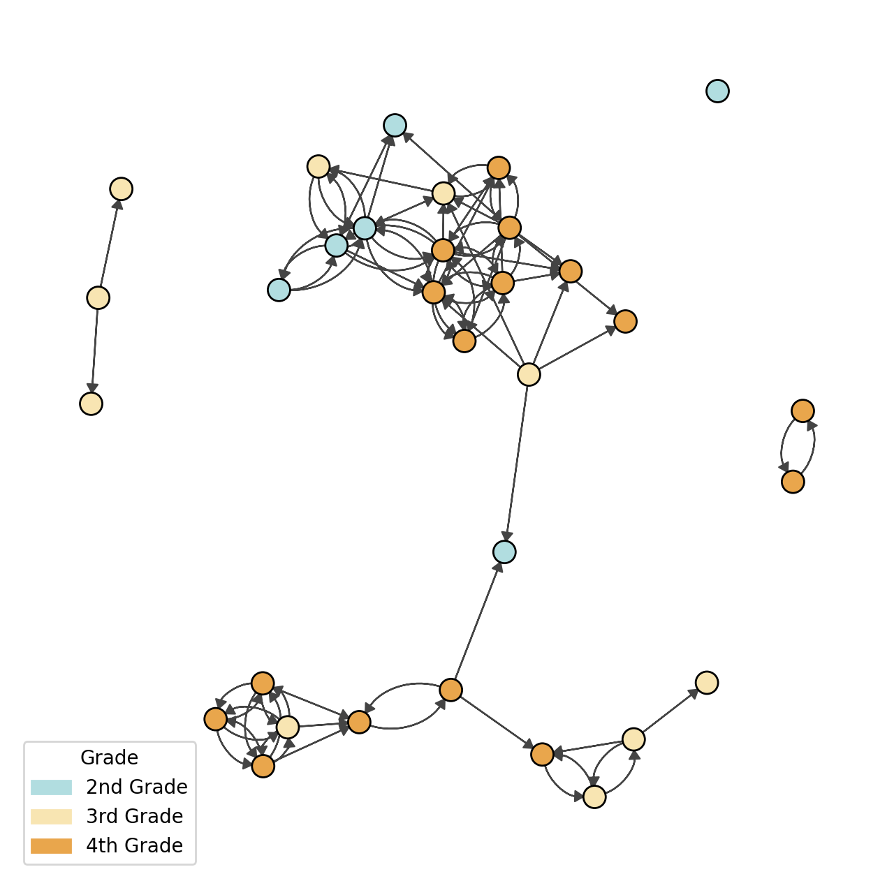
We can call the function to calculate the group level or the network level score.

grades_group_level = coleman(membership= "grade", graph = g) # Group level 
print(grades_group_level)

[np.float64(0.40384615384615385), np.float64(0.1711229946524064), np.float64(0.4976851851851852)]

grade_network_level = coleman(membership= "grade", graph = g, network_level= True)
print(grade_network_level)

0.4002418379685611

References

• Bojanowski, M., & Corten, R. (2014). Measuring segregation in social networks. Social networks, 39, 14-32.

• Coleman, James S. “Relational analysis: The study of social organizations with survey methods.” Human organization 17.4 (1958): 28-36.

• Van de Bunt, G. G., van Duijn, M. A. J., & Snijders, T. A. B. (1999). Friendship networks through time: An actor-oriented statistical network model. Computational and Mathematical Organization Theory, 5, 167-192