Krackhardt’s EI Score

EI index (Krackhard & Stern, 1988) is a particularly simple approach to quantify segregation in social networks. It is especially popular due to its early adoptation. EI index is defined originally as,

\[ S_{EI} = \frac{EL - IL}{EL + IL}\]

Where \(EL\) is the “external links”, links running between the groups, and \(IL\) is the “internal links”, links running within the groups.

import igraph as ig 
import random 
import matplotlib.pyplot as plt 
import matplotlib.patches as mpatches
from netseg import krackhardt_ei


%config InlineBackend.figure_format = 'retina'

COLORS = [
    '#2C486F',
    '#436796',
    '#5E8FAE',
    '#80BDD6',
    '#B1DDE0',
    "#fdf8e7",
    '#F8E5B2',
    '#F3CF63',
    '#E9A64C',
    '#E3843B',
    '#DA584E'
 ]

def make_symmetric_sbm(p_in, p_out, n_groups, nodes_per_group, membership, **kwargs):
    pref_matrix = [
        [p_in if i == j else p_out for j in range(n_groups)] 
        for i in range(n_groups)
    ]
    block_sizes = [nodes_per_group] * n_groups
    g = ig.Graph.SBM(pref_matrix, block_sizes, **kwargs)
    
    g.vs['membership'] = membership
    
    return g 

Basic Usage

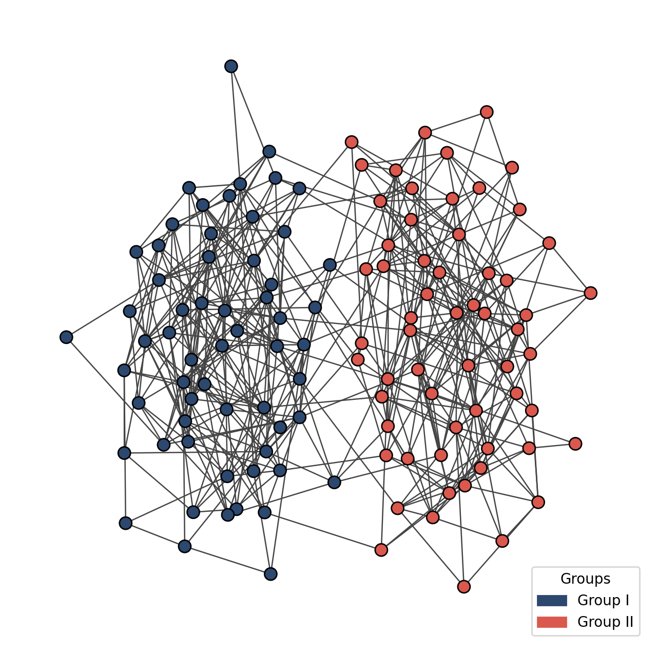
It is pretty straightforward to use EI index.

random.seed(7)
membership = [0 if i < 60 else 1 for i in range(120)]
g = make_symmetric_sbm(0.12, 0.006, 2, 60, membership)

fig, ax = plt.subplots(figsize = (8,8))
ig.plot(g,
        vertex_color = [COLORS[0] if i == 0 else COLORS[-1] for i in membership],
        layout = g.layout_kamada_kawai(),
        edge_width = .9,
        vertex_size = 24,
        target = ax)

g1_patch = mpatches.Patch(color=COLORS[0], label='Group I')
g2_patch = mpatches.Patch(color=COLORS[-1], label='Group II')
ax.legend(handles=[g1_patch, g2_patch], loc='lower right', title="Groups")
plt.show()

ei_score = krackhardt_ei("membership", g)
print(ei_score)

-0.8796296296296297

It is important to notice that for more segregated networks metric will return lower values.

Multiple Groups

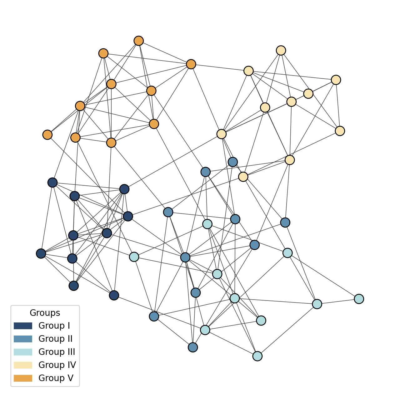
It is possible to apply the metric for multiple groups.

labels = ["Group I", "Group II", "Group III", "Group IV", "Group V"]
base_colors = [COLORS[i * 2] for i in range(5)] 

membership = [labels[i // 10] for i in range(50)]
v_colors = [base_colors[i // 10] for i in range(50)]

random.seed(4)
fig, ax = plt.subplots(figsize=(8, 8))
g_multiple = make_symmetric_sbm(0.5, 0.03, 5, 10, membership)

ig.plot(
    g_multiple,
    vertex_color=v_colors,
    target=ax,
    vertex_size=30,
    edge_width=0.6,
    layout=g_multiple.layout_kamada_kawai(),
)

patches = [mpatches.Patch(color=c, label=l) for c, l in zip(base_colors, labels)]
ax.legend(handles=patches, loc='lower left', title="Groups")
plt.show()

ei_score_multiple = krackhardt_ei("membership",g_multiple)
print(ei_score_multiple)

-0.6026490066225165

Example

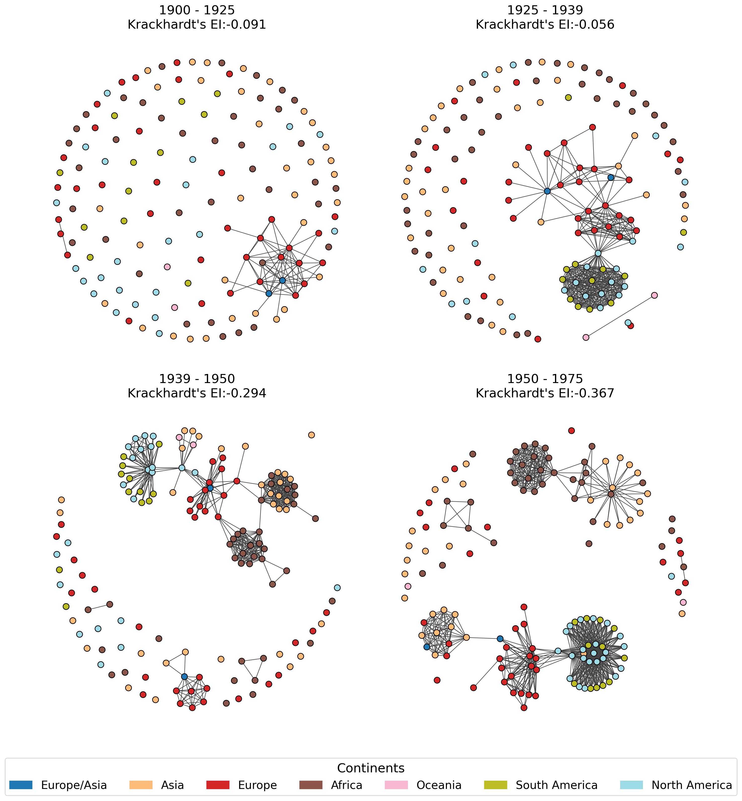
To demonstrate the EI index, we are using the Correlates of War, Formal Alliances dataset (v4.1). We are only considering the undirected network with defense pacts, which is the highest level of military commitment, requiring alliance members to come to each other’s aid militarily if attacked by a third party (Gibler, 2009). The exogenous property of a node is the continent that a country resides in. For demonstration purposes, we are only focusing on the quarters of the 20th Century.

g_alliances = ig.Graph.Read_GML('../assets/cowfad/cowfad_graph.gml')

continents = list(set(g_alliances.vs['continent']))
tab20 = plt.get_cmap('tab20', len(continents))
color_mapping = {cont: tab20(i) for i, cont in enumerate(continents)}


fig, axs = plt.subplots(2, 2, figsize=(14, 16))
axs = axs.flatten()
years = ["1900 - 1925", "1925 - 1939", "1939 - 1950","1950 - 1975"]
for idx, period in enumerate([1, 2, 3, 4]):
    

    edges_in_period = g_alliances.es.select(period=period)
    sub_g = g_alliances.subgraph_edges(edges_in_period, delete_vertices=False)
    v_colors = [color_mapping[c] for c in sub_g.vs['continent']]
    ei  = krackhardt_ei("continent", sub_g)
    ig.plot(
        sub_g,
        vertex_size=24,
        vertex_color=v_colors,
        layout=sub_g.layout_kamada_kawai(),
        target=axs[idx],
        edge_width=0.8
    )
    
    axs[idx].set_title(f"{years[idx]}\nKrackhardt's EI:{ei:.3f}", fontsize=18)
    axs[idx].axis('off') 

legend_patches = [mpatches.Patch(color=color_mapping[c], label=c) for c in continents]
fig.legend(
    handles=legend_patches, 
    loc='lower center', 
    ncol=len(continents), 
    title="Continents", 
    fontsize=16, 
    title_fontsize=18
)

fig.tight_layout()
plt.subplots_adjust(bottom=0.08) 
plt.show()

References

• Krackhardt, David, and Robert N. Stern. “Informal networks and organizational crises: An experimental simulation.” Social psychology quarterly (1988): 123-140.