Gupta, Anderson and May’s Q

Gupta, Anderson and May’s Q (GAMQ) (Gupta, 1989) is designed for undirected networks and it is based on the contact layer of the mixing matrix (Bojanowski, 2014). If we define \(f_{gh}\) as the the mixing matrix that contains the proportion of ties of actors in group \(g\) to actors in group \(h\),

\[GAMQ = \frac{\sum^K_{g = 1} \lambda_g - 1}{K - 1} \]

where \(\lambda_g\) are the eigenvalues of the matrix \([f_{gh}]\). Without decomposition, since sum of the eigenvalues of a square matrix of real or complex numbers is equal to its trace (Harville, 1997), we can rewrite the equation as,

\[GAMQ = \frac{\sum^K_{g = 1} f_{gg} - 1}{K - 1} \]

where \(\sum^K_{g = 1} f_{gg}\) is the trace of the matrix. Measure varies in between \(-1 / (K-1)\) (maximal integration) and \(1\) (maximal segregation).

from netseg import gamix
import igraph as ig 
import numpy as np 
import random 
from time import perf_counter
import itertools

import matplotlib.pyplot as plt 
from matplotlib.ticker import FormatStrFormatter
from matplotlib.colors import LinearSegmentedColormap, to_hex, Normalize, BoundaryNorm
import matplotlib.lines as mlines
from mpl_toolkits.axes_grid1 import make_axes_locatable
from matplotlib.cm import ScalarMappable
import matplotlib.patches as mpatches

%config InlineBackend.figure_format = 'retina'

COLORS = [
    '#2C486F',
    '#436796',
    '#5E8FAE',
    '#80BDD6',
    '#B1DDE0',
    "#fdf8e7",
    '#F8E5B2',
    '#F3CF63',
    '#E9A64C',
    '#E3843B',
    '#DA584E'
 ]

def make_symmetric_sbm(p_in, p_out, n_groups, nodes_per_group, membership, **kwargs):
    pref_matrix = [
        [p_in if i == j else p_out for j in range(n_groups)] 
        for i in range(n_groups)
    ]
    block_sizes = [nodes_per_group] * n_groups
    g = ig.Graph.SBM(pref_matrix, block_sizes, **kwargs)
    
    g.vs['membership'] = membership
    
    return g 


membership = [1 if i < 10000 else 0 for i in range(20000)]
g = make_symmetric_sbm(0.05, 0.008, 2, 10000, membership)
gamix("membership",g)

np.float64(0.723935363436615)

Basic Usage

You can directly calculate GAMQ with the function gamix.

random.seed(5)
membership = [0 if i < 100 else 1 for i in range(200)]
g = make_symmetric_sbm(0.05, 0.001, 2, 100, membership)



fig, ax = plt.subplots(figsize = (8,8))

ig.plot(g, 
        vertex_size = 36,
        edge_color = "black",
        edge_width = 0.6,
        vertex_color = [COLORS[-1] if i  == 1 else COLORS[0] for i in membership],
        layout = g.layout_kamada_kawai(),
        target = ax)

g1 = mpatches.Patch(color = COLORS[-1], label = "Group I")
g2 = mpatches.Patch(color = COLORS[0], label = "Group II")

ax.legend(handles = [g1,g2], loc = "lower right", title = "Nodal Attributes")
plt.show()

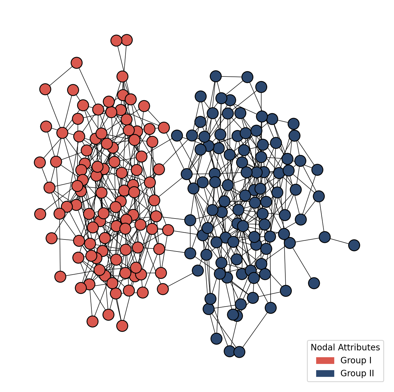
gamix_score = gamix("membership", g)
print(gamix_score)

0.9661550570641482

Multiple Groups

GAMQ can easily be applied to multiple groups.

random.seed(5)
membership = [0] * 30 + [1] * 30  + [2] * 30
g_multiple = make_symmetric_sbm(0.22, 0.007, 3, 30, membership)

fig, ax = plt.subplots(figsize = (8,8))

ig.plot(g_multiple, 
        vertex_size = 36,
        edge_color = "black",
        edge_width = 0.6,
        vertex_color = [COLORS[(i + 1) * 3] for i in membership],
        layout = g_multiple.layout_kamada_kawai(40000),
        target = ax)

g1 = mpatches.Patch(color = COLORS[3], label = "Group I")
g2 = mpatches.Patch(color = COLORS[6], label = "Group II")
g3 = mpatches.Patch(color = COLORS[9], label = "Group II")

ax.legend(handles = [g1,g2,g3], loc = "lower right", title = "Nodal Attributes")
plt.show()

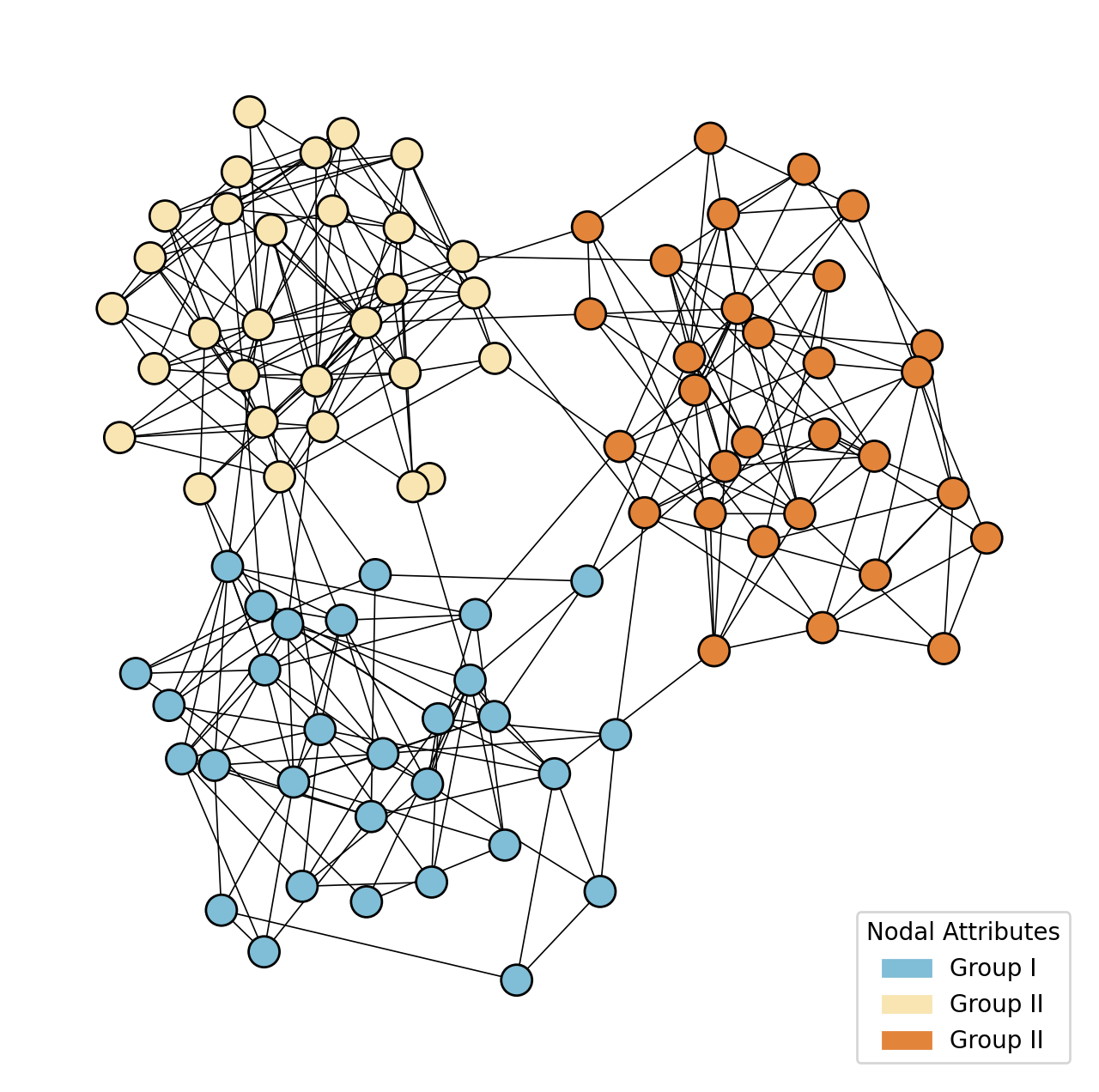
gamq_score = gamix(membership, g_multiple)
print(gamq_score)

0.8962974567024622

Example

We use the “Hartford Drug Users” dataset to demonstrate the GAMQ. Edges indicate acquaintanceship between individuals based on ethnographic observations. We measure the segregation with the nodal attribute “ethnicity”, which is grouped into three categories: Whites/Others, African Americans, and Puerto Ricans/Latinos. Original dataset can be found here.

COLORS = [
    "#9B4D2E",  
    "#A8952A", 
    "#2A5C4A"]
g_example = ig.Graph.Read_GML('../assets/drugs/drug_use.gml')
ethn_dict = {2:"African American", 3:"Puerto Rican/Latino"}
g_example.vs['Ethnicity'] = [ethn_dict.get(i, "Other") for i in g_example.vs['Ethnicity']]
colors_dict = dict(zip(set(g_example.vs['Ethnicity']),COLORS))

fig, ax = plt.subplots(figsize = (8,8))
random.seed(2)
ig.plot(g_example,
        layout = g_example.layout_fruchterman_reingold(),
        vertex_color = [colors_dict[i] for i in g_example.vs['Ethnicity']],
        target = ax,
        edge_width = 0.9,
        vertex_size = 16)

w_patch = mpatches.Patch(color = COLORS[0], label = "White/Other")
aa_patch = mpatches.Patch(color = COLORS[1], label = "African American")
l_patch = mpatches.Patch(color = COLORS[2], label = "Puerto Rican/Latino")
ax.legend(handles= [w_patch, aa_patch, l_patch], title = "Ethnicity", loc = "lower right")
plt.show()

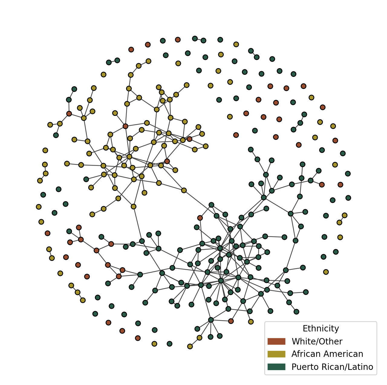
gamq_score_drug = gamix("Ethnicity", g_example)
print(gamq_score_drug)

0.6138075011558022

References

• Bojanowski, M., & Corten, R. (2014). Measuring segregation in social networks. Social networks, 39, 14-32.

• Gupta, Sunetra, Roy M. Anderson, and Robert M. May. “Networks of sexual contacts: implications for the pattern of spread of HIV.” Aids 3.12 (1989): 807-818.