Moran’s I
Originally applied to measure spatial auto-correlation, Moran’s I can easily be applied to networks since the original setting the metric is introduced can be represented as a 2-D regular lattice. Although netseg uses the direct neighbors, there are additional ways to extend the metrics, defining complex neighborhood relationships between the nodes. For a detailed explanation see Analytic Methods for
Measuring Network Segregation by James M. Murphy or Measuring Segregation via Analysis on Graphs by Duchin et al.
Moran’s I can be calculated with:
Where \(N\) is the number of nodes in the network, \(S_0\) is the sum of the values in the adjacency matrix (applicable in case of a weighted network), \(x\) is the value of interest. \(w_{ij}\) is basically the value within the adjacency matrix at row \(i\) and column \(j\).
Moran’s \(I\) is evaluated as a test of the null hypothesis that the nodal attribute is arranged at random with respect to the graph structure, but the two branches of the function realize this test differently. When no null models are supplied, the function relies on the closed-form randomization moments: the statistic is standardized to
and referred to a standard normal distribution, with the two sided \(p\)-value obtained as \(\mathrm{erfc}(|z| / \sqrt{2})\) this is an asymptotic \(z\)-test whose normal approximation is justified only for sufficiently large \(N\) and moderate attribute kurtosis, which is why the variance is left undefined below four nodes. When null models are supplied, the function instead constructs the null distribution empirically from the ensemble of statistics and reports the \(p\)-value as the two sided empirical tail, so that no distributional assumption is imposed; the accompanying \(z\)-score is retained only as a descriptive standardization and is not the basis of the empirical \(p\)-value. Both options therefore test the same hypothesis, differing in whether the reference distribution is the asymptotic normal or the supplied ensemble itself.
Documentation shows the metric’s implementation on various examples; for undirected network examples with discrete and non-discrete attributes you can see the first two examples (your network does not have to be a lattice, a lattice is given since it is a common demonstration). You can also apply the metric also on directed, weighted or both type of networks. Finally, we are evaluating the meaning of the p-value and supplying our own null models.
from netseg import moran_i

import igraph as ig
import matplotlib.pyplot as plt
from matplotlib.colors import LinearSegmentedColormap, to_hex, Normalize, ListedColormap
import numpy as np
from matplotlib.cm import ScalarMappable
from matplotlib.lines import Line2D
import random
random.seed(2)


%config InlineBackend.figure_format = 'retina'
plt.rcParams.update({
    "font.family": "serif",
    "mathtext.fontset": "cm",
    "font.size": 11,
    "axes.linewidth": 1.0,
    "xtick.direction": "in",
    "ytick.direction": "in",
    "xtick.top": True,
    "ytick.right": True,
    "xtick.minor.visible": True,
    "ytick.minor.visible": True,
})

COLORS_DIV = [
    '#2C486F',
    '#436796',
    '#5E8FAE',
    '#80BDD6',
    '#B1DDE0',
    "#fdf8e7",
    '#F8E5B2',
    '#F3CF63',
    '#E9A64C',
    '#E3843B',
    '#DA584E'
 ]

COLORS_NDIV = [
    '#1C1044',
    '#4F1078',
    '#812581',
    '#B63679',
    '#E75263',
    '#F98C51',
    '#FEC98D'
]


def get_custom_colors_hex(values, COLORS_DIV = COLORS_DIV):
    vmin = min(values)
    vmax = max(values)

    norm = Normalize(vmin=vmin, vmax=vmax)
    custom_cmap = LinearSegmentedColormap.from_list("custom_gradient", COLORS_DIV)

    return [to_hex(custom_cmap(i)) for i in norm(values)]

def make_symmetric_sbm(p_in, p_out, n_groups, nodes_per_group, attribute_g1_m, attribute_g2_m, attribute_g1_std, attribute_g2_std, **kwargs):
    pref_matrix = [
        [p_in if i == j else p_out for j in range(n_groups)]
        for i in range(n_groups)
    ]
    block_sizes = [nodes_per_group] * n_groups
    g = ig.Graph.SBM(pref_matrix, block_sizes, **kwargs)

    g.vs['attribute'] = np.append(np.random.normal(attribute_g1_m,
                                                   attribute_g1_std,
                                                   size = g.vcount() // 2),
                                                   np.random.normal(attribute_g2_m,
                                                   attribute_g2_std,
                                                   size = g.vcount() // 2))

    return g
Usage Examples
Since the metric is originally designed for 2D lattices, we first demonstrate the behaviour of the metrics with a 2D lattice that the variable of interest is positioned in a varying manner and with different values.
Ising Model on a 2D Square Lattice
The Ising model is one of the best-known models in physics, describing ferromagnetism in statistical mechanics. In this demonstration we are not going to dive deep into the Ising model itself, since that is well beyond the scope of a package demo. We only use it as a generator: a source of spatially structured configurations on which we investigate how Moran’s I behaves.
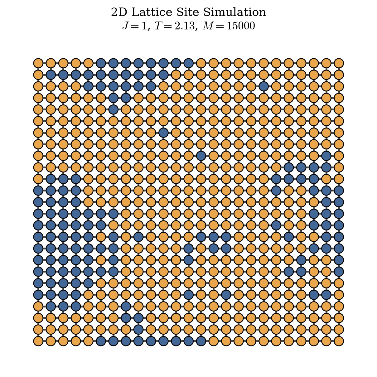
We use a Monte Carlo scheme with the Metropolis acceptance rule to evolve the lattice from a random initialization toward configurations with spatial structure, domains (“islands”) of aligned spins. If you want to learn more about the sampling method and the model itself, the following are good introductory sources for both implementation and theory: [1], [2], [3].
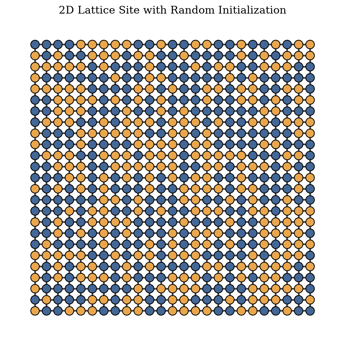
Algorithmically, we start with an \(N \times N\) lattice, randomly initialized, where each site takes a value in \(\{-1, +1\}\). The system energy is the standard Ising Hamiltonian \(H = -J \sum_{\langle i,j \rangle} s_i s_j\), summed over nearest-neighbour pairs. We then update the spins via single-spin-flip dynamics.
For \(M\) steps:
1 - Pick a random site and propose flipping its spin.
2 - Compute the energy difference \(\Delta H\) induced by the flip.
2.1 - If \(\Delta H < 0\), accept the flip.
2.2 - If \(\Delta H \geq 0\), accept the flip with probability \(p = \exp\!\left(-\dfrac{\Delta H}{k_B T}\right)\).
Here \(\Delta H\) is the energy difference, \(T\) is the temperature, \(J\) is the coupling constant and \(k_B\) is the Boltzmann constant. For the lattice below, we impose periodic boundary conditions, which topologically identify the lattice with a torus, so that sites on opposite edges interact as nearest neighbours.
g = ig.Graph.Lattice(dim = [25,25],
                     directed= False,
                     circular = True) # the default is True, periodic boundary conditions (wraps into a torus)

# We can test whether wrapped into a torus with
assert 25 ** 2 * 4 == g.ecount() * 2 # Since igraph does not count twice
state_color = {-1: '#436796', 1: '#E9A64C'}

generator = np.random.default_rng(33)
states = generator.choice([-1,1], g.vcount(), replace= True)

g.vs['state'] = states
fig, ax = plt.subplots(figsize = (6,6))
ig.plot(g,
        layout = g.layout_grid(),
        vertex_color = [state_color[i] for i in g.vs['state']],
        target = ax)
ax.set_title('2D Lattice Site with Random Initialization', pad= 0.1)
fig.tight_layout(pad = 0.5)
plt.show()
from math import exp
class MC_Metropolis:

  def __init__(self,
               graph:ig.Graph,
               temperature:float,
               coupling:float,
               seed:int = 33):

    self.graph = graph.copy()
    self.temperature = temperature
    self.coupling = coupling
    # Since each probability is predefine, we can calculate it as lookup
    # instead of calculating it at each iteration.

    self.delta_lookup = {
        s_times_S: exp((-2 * self.coupling * s_times_S) / self.temperature)
        for s_times_S in (-4, -2, 0, 2, 4)
    }


    self.seed = seed
    self.rng = np.random.default_rng(self.seed)

  def __repr__(self):

    return f"Ising model simulation with the embedded graph at {hex(id(self.graph))} at {hex(id(self))}."

  def offer(self,sums:np.ndarray):

    return np.array([self.delta_lookup[i] for i in sums])


  def sweep(self, step=10000):
      self.graph
      states = np.array(self.graph.vs['state'])
      neighbors = [self.graph.neighbors(i) for i in range(self.graph.vcount())]

      picked_sites = self.rng.choice(self.graph.vcount(), replace=True, size=step)

      for i in picked_sites:
          s_times_S = states[i] * states[neighbors[i]].sum()
          if self.rng.random() < self.delta_lookup[s_times_S]:
              states[i] = -states[i]

      self.graph.vs['state'] = states.tolist()
simulation = MC_Metropolis(g, 2.13, 1)
simulation.sweep(15000)
state_color = {-1: '#436796', 1: '#E9A64C'}

fig, ax = plt.subplots(figsize = (6,6))
ig.plot(simulation.graph,
        layout = simulation.graph.layout_grid(),
        vertex_color = [state_color[i] for i in simulation.graph.vs['state']],
        target = ax)
ax.set_title(f"2D Lattice Site Simulation\n" + r"$J = 1$, $T=2.13$, $M = 15000$", pad= 0.1)
fig.tight_layout(pad = 0.5)
plt.show()
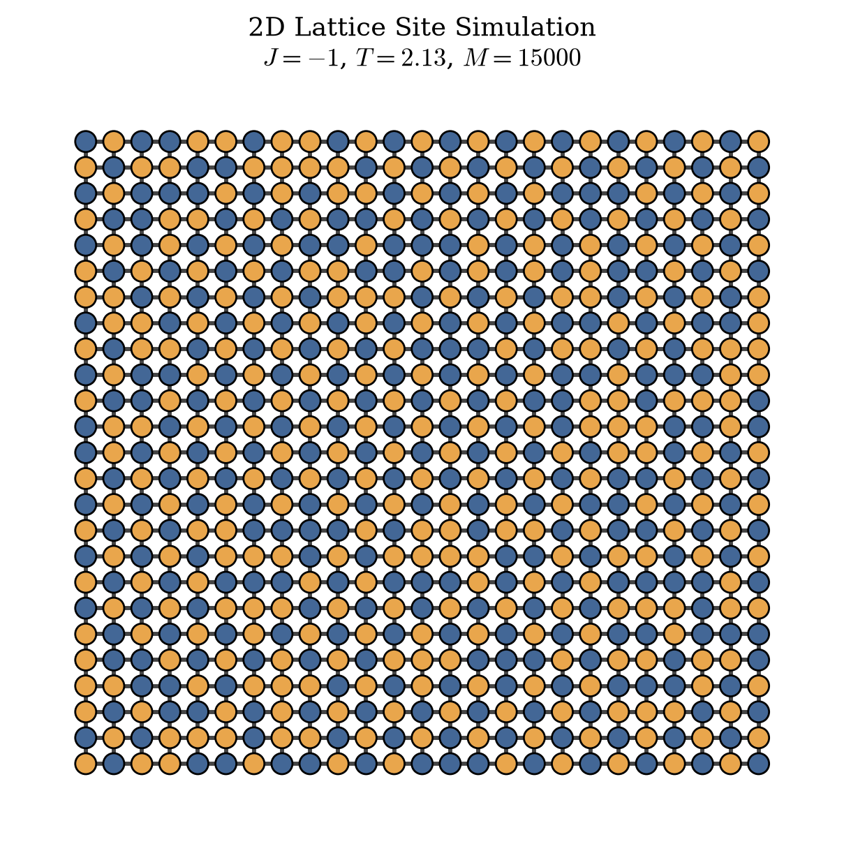
If \(J\) was negative it would favor the anti-aligned neighborhors
simulation = MC_Metropolis(g, 2.13, -1)
simulation.sweep(15000)

state_color = {-1: '#436796', 1: '#E9A64C'}

fig, ax = plt.subplots(figsize = (6,6))
ig.plot(simulation.graph,
        layout = simulation.graph.layout_grid(),
        vertex_color = [state_color[i] for i in simulation.graph.vs['state']],
        target = ax)
ax.set_title(f"2D Lattice Site Simulation\n" + r"$J = -1$, $T=2.13$, $M = 15000$", pad= 0.1)
fig.tight_layout(pad = 0.5)
plt.show()
Now we can observe how Moran’s I behaves in this model with the following approach.
The graph will be, coupling strength -1 and +1, temperature changes, then we are going to show Moran’s I and how it behaves across each 100 iteration.
g = ig.Graph.Lattice(dim = [25,25],
                     directed= False,
                     circular = True)

states = generator.choice([-1,1], g.vcount(), replace= True)


results = np.zeros(shape = (150, 20))

for index, temperature in enumerate(np.linspace(0.5,5,20)):
  observed_statistics = []
  g.vs['state'] = states
  simulation = MC_Metropolis(g, temperature, 1) # Positive coupling


  for i in range(150):

    observed_statistic, _, _, _, _ = moran_i(simulation.graph.vs['state'], simulation.graph)
    observed_statistics.append(observed_statistic)
    simulation.sweep(100)


  results[:,index] = observed_statistics

g = ig.Graph.Lattice(dim = [25,25],
                     directed= False,
                     circular = True)

states = generator.choice([-1,1], g.vcount(), replace= True)


results_neg = np.zeros(shape = (150, 20))

for index, temperature in enumerate(np.linspace(0.5,5,20)):
  observed_statistics_neg = []
  g.vs['state'] = states
  simulation = MC_Metropolis(g, temperature, -1) # negative coupling


  for i in range(150):

    observed_statistic, _, _, _, _ = moran_i(simulation.graph.vs['state'], simulation.graph)
    observed_statistics_neg.append(observed_statistic)
    simulation.sweep(100)


  results_neg[:,index] = observed_statistics_neg
temperatures = np.linspace(0.5, 5, 20)
palette = get_custom_colors_hex(temperatures)

fig, ax = plt.subplots(figsize=(8, 6))
iterations = np.arange(results.shape[0])
for i in range(results.shape[1]):
    ax.plot(results[:, i], c=palette[i],
                   alpha = .6, markevery= 5,
                   marker = "o", markersize = 5)
    ax.plot(results_neg[:, i], c=palette[i],
                       alpha = .6, markevery = 5,
                       marker = "s", markersize = 5)

ax.set_xlabel(r"Iteration ($\times 100$)")
ax.set_ylabel(r"Moran's $I$")

ax.tick_params(which="both", length=4, width=1.0)
ax.tick_params(which="major", length=6)

cmap = ListedColormap(palette)
norm = Normalize(vmin=temperatures.min(), vmax=temperatures.max())
sm = ScalarMappable(cmap=cmap, norm=norm)

cbar = fig.colorbar(sm, ax=ax, pad=0.02)
cbar.set_label(r"Temperature $T$")

coupling_handles = [
    Line2D([], [], marker="o", linestyle="none", color="0.3", label=r"$J = +1$ (Positive Coupling)"),
    Line2D([], [], marker="s", linestyle="none", color="0.3", label=r"$J = -1$ (Negative Coupling)"),
]
ax.legend(handles=coupling_handles, frameon=False, loc="best")

fig.tight_layout()
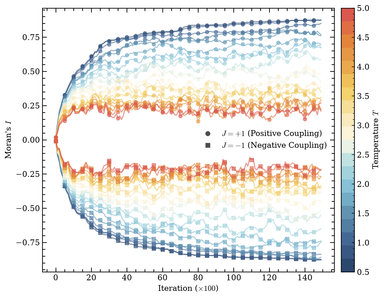
We measure Moran’s \(I\) on the lattice as the Ising dynamics run, for 20 temperatures and both signs of the coupling. Each curve is one temperature. Color encodes \(T\), dark blue for cold and red for hot. Circles mark the ferromagnetic runs (\(J=+1\)) and squares the antiferromagnetic ones (\(J=-1\)). We sample \(I\) every 100 sweeps, which is why the \(x\)-axis is in units of \(\times 100\).
Both families start at \(I \approx 0\), which is what we want to see. The random initialization has no spatial structure, so a spatial autocorrelation statistic should read roughly zero. From there the two signs of \(J\) pull apart in opposite directions, and this split is the entire point of the demo.
The \(J=+1\) runs climb to \(I > 0\). Neighbours want to align, aligned domains form, and Moran’s \(I\) picks up that positive autocorrelation directly. The \(J=-1\) runs fall to \(I < 0\). Here the coupling favours anti-aligned neighbours, the lattice settles into a checkerboard, and \(I\) reports the negative autocorrelation. So the sign of \(I\) recovers the sign of the coupling without ever being told about it. It reads the structure off the field alone, which is exactly the behaviour we would want from the statistic on real segmentation data.
Temperature controls how far \(|I|\) gets to travel. The cold runs (dark blue) saturate near \(\pm 0.9\), strong order in either the aligned or checkerboard sense. As \(T\) rises the plateaus shrink, and the hottest runs (red) settle around \(\pm 0.25\). That is the disordered regime, where thermal fluctuations dominate the coupling, order is short-ranged, and \(I\) stays small. The hot runs plateau near \(\pm 0.25\) rather than at \(0\) for two reasons. Part of it is residual short-range correlation, since we only reach about \(2\,T_c\) rather than infinite temperature. Part of it is the finite-size spread of \(I\) on a \(25 \times 25\) lattice. Both branches relax within the first ~25 samples and then fluctuate around their equilibrium value, which is the signature of a chain that has equilibrated.
Gaussian Random Field (GRF) on a 2D Square Lattice
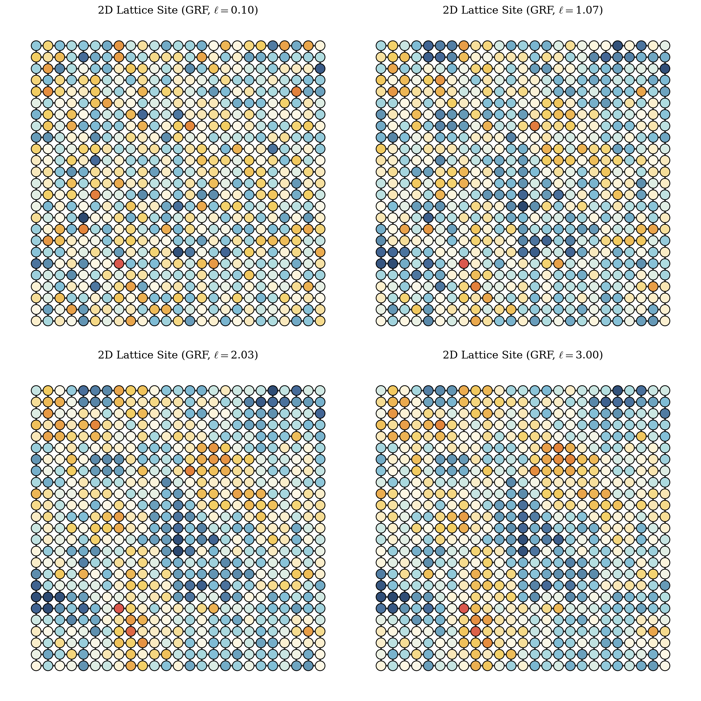
The GRF is the standard model for spatial autocorrelation in statistics, and unlike the Ising model it produces continuous values rather than discrete spins. We use it here for the same reason we used the Ising model, as a generator of spatially structured fields on which to watch how Moran’s I behaves. This time the structure is a smooth gradient rather than sharp domains, which lets us test the statistic on graded data instead of a two-state field. The canonical reference for this framework is Cressie, Statistics for Spatial Data (Wiley, 1993).
The idea is that the entire vector of node values \(\mathbf{z} = (z_1, \dots, z_n)\) is drawn from a single multivariate normal distribution,
All of the spatial structure lives in the covariance matrix \(\Sigma\), which sets how correlated every pair of nodes is. We define each entry as a function of the distance \(d_{ij}\) between nodes \(i\) and \(j\) using an exponential kernel,
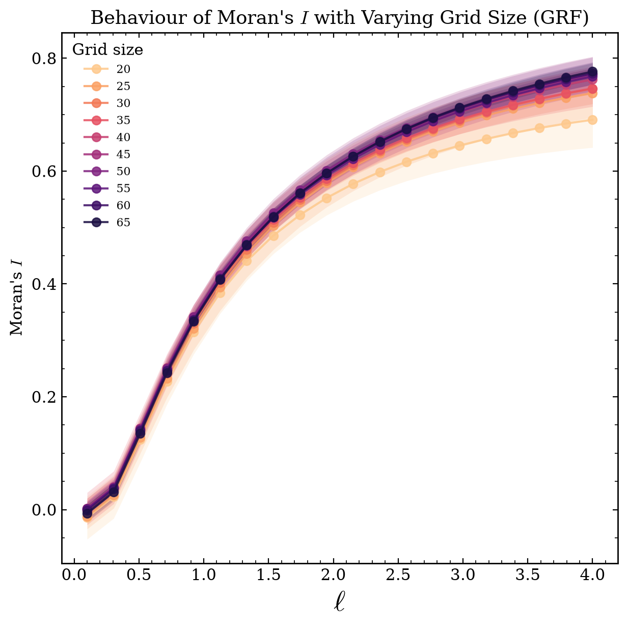
where \(\sigma^2\) is the overall variance and \(\ell\) is the correlation length. The correlation length is our one knob, analogous to temperature in the Ising demo. A small \(\ell\) makes correlation die off almost immediately, so the field looks like white noise and Moran’s I stays near zero. A large \(\ell\) extends correlation across many nodes, so the field becomes a smooth gradient and Moran’s I approaches one.
To sample the field we factor the covariance with a Cholesky decomposition \(\Sigma = L L^\top\), draw a vector of independent standard normals \(\mathbf{u} \sim \mathcal{N}(\mathbf{0}, I)\), and set \(\mathbf{z} = L \mathbf{u}\). The result has exactly the covariance \(\Sigma\) we specified. On a \(25 \times 25\) lattice \(\Sigma\) is \(625 \times 625\), so this factorization is cheap. We add a small constant \(\varepsilon\) to the diagonal of \(\Sigma\) before factoring, which keeps it positive definite against numerical round-off and also models fine-scale noise.
import numpy as np

class GaussianRandomField:

    def __init__(self,
                 graph: ig.Graph,
                 correlation_length: float,
                 variance: float = 1.0,
                 nugget: float = 1e-8,
                 seed: int = 33):

        self.graph = graph.copy()
        self.correlation_length = correlation_length
        self.variance = variance
        self.nugget = nugget

        self.seed = seed
        self.rng = np.random.default_rng(self.seed)

        # lookup we build it once in the constructor and reuse it every sample.
        distances = self._pairwise_distances()
        covariance = self.variance * np.exp(-distances / self.correlation_length)
        covariance += self.nugget * np.eye(self.graph.vcount())

        self.cholesky_factor = np.linalg.cholesky(covariance)

    def __repr__(self):
        return (f"Gaussian random field with the embedded graph at "
                f"{hex(id(self.graph))} at {hex(id(self))}.")

    def _pairwise_distances(self):
        """
        We need to keep the Torus structure but avoid hop-distance,
        so we wrap the coordinates around, if it passes halfway, we
        wrap it around.
        """

        coordinates = np.array(self.graph.layout_grid().coords)
        grid_size = np.sqrt(self.graph.vcount())

        differences = np.abs(coordinates[:, None, :] - coordinates[None, :, :])
        differences = np.minimum(differences, grid_size - differences)  # wrap each axis
        return np.sqrt((differences ** 2).sum(axis=-1))

    def sample(self):
        standard_normals = self.rng.standard_normal(self.graph.vcount())
        field_values = self.cholesky_factor @ standard_normals

        self.graph.vs['state'] = field_values.tolist()
        return field_values
g = ig.Graph.Lattice(dim = [25,25],
                        directed= False,
                        circular = True)
fig, axs = plt.subplots(2,2,figsize = (12,12))
axs = axs.flatten()
for index, corr_length in enumerate(np.linspace(0.1,3,4)):

        grf = GaussianRandomField(g, corr_length)
        attr = grf.sample()
        g.vs['attribute'] = attr

        ig.plot(g,
                layout = g.layout_grid(),
                vertex_color = get_custom_colors_hex(g.vs['attribute']),
                target = axs[index],
                vertex_size = 34)
        axs[index].set_title(f"2D Lattice Site (GRF, " + r"$\ell = $" + f"{corr_length:.2f})", pad= 0.1)

fig.tight_layout(pad = 0.01)
plt.show()
We can observe the behaviour of Moran’s I regarding the correlation length with the following approach.
grid_sizes = range(20, 70, 5)
ell_values = np.linspace(0.1, 4, 20)
n_repeats = 10

results = np.zeros(shape=(len(ell_values), len(grid_sizes), n_repeats))

for size_index, g_size in enumerate(grid_sizes):
    g = ig.Graph.Lattice(dim=[g_size, g_size], directed=False, circular=True)

    for ell_index, ell in enumerate(ell_values):
        for repeat_index in range(n_repeats):

            seed = repeat_index
            grf = GaussianRandomField(g, ell, seed=seed)
            attribute_values = grf.sample()
            g.vs['attribute'] = attribute_values
            observed_statistic, _, _, _, _ = moran_i(attribute='attribute', graph=g)
            results[ell_index, size_index, repeat_index] = observed_statistic

results_mean = results.mean(axis=2)
results_std = results.std(axis=2)
fig, ax = plt.subplots(figsize=(6, 6))
palette_ndiv = get_custom_colors_hex(grid_sizes, COLORS_NDIV[::-1])

for size_index, size in enumerate(grid_sizes):
    mean_curve = results_mean[:, size_index]
    std_curve = results_std[:, size_index]

    ax.plot(ell_values, mean_curve, marker="o", markevery=1, alpha=0.85,
            c=palette_ndiv[size_index], label=f"{size}")
    ax.fill_between(ell_values, mean_curve - std_curve, mean_curve + std_curve,
                    color=palette_ndiv[size_index], alpha=0.18, linewidth=0)

ax.set_xlabel(r'$\ell$', fontdict={"fontsize": 20})
ax.set_ylabel("Moran's " + r'$I$')
ax.set_title("Behaviour of Moran's " + r"$I$" + " with Varying Grid Size (GRF)")
ax.legend(title="Grid size", frameon=False, fontsize=8)
fig.tight_layout(pad=0.1)
plt.show()
Directed Networks
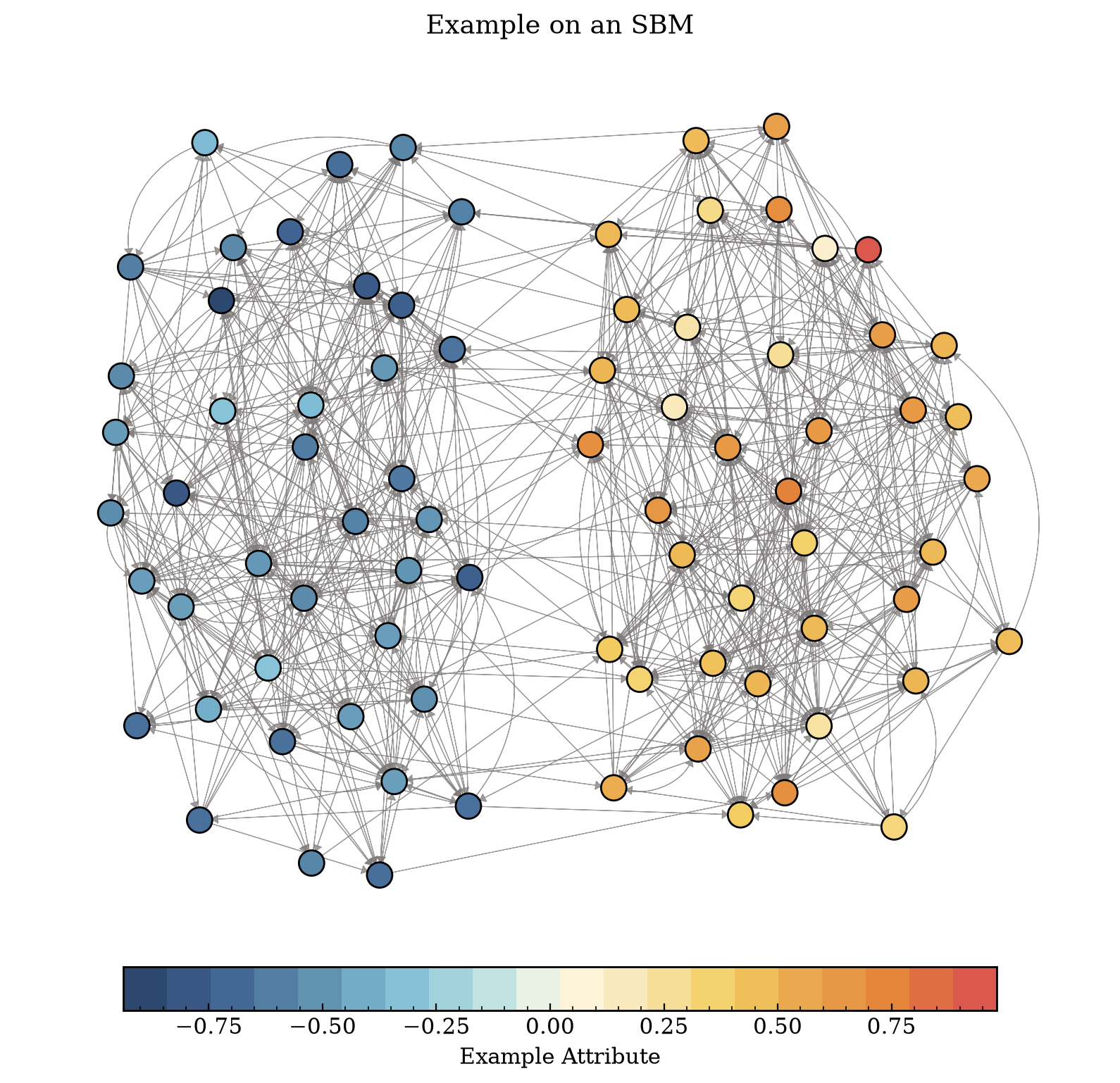
In here we are demonstrating the behaviour of the metric with a stochastic block model.
g = make_symmetric_sbm(0.2, 0.02, 2, 40, .6, -.6, .2 , .2, directed = True)
fig, ax = plt.subplots(figsize = (10,10))
ig.plot(g,
        target = ax,
        vertex_size = 36,
        edge_width = .4,
        edge_arrow_width = 12.3,
        edge_arrow_size = 8,
        edge_color = "#807C7CC3",
        vertex_color = get_custom_colors_hex(g.vs['attribute']))

ax.set_title('Example on an SBM')
cmap = ListedColormap(palette)
norm = Normalize(vmin=min(g.vs['attribute']), vmax=max(g.vs['attribute']))
sm = ScalarMappable(cmap=cmap, norm=norm)

cbar = fig.colorbar(sm, ax=ax, pad=0.01, orientation = "horizontal",
                    shrink = .8)
cbar.set_label(r"Example Attribute")
plt.show()
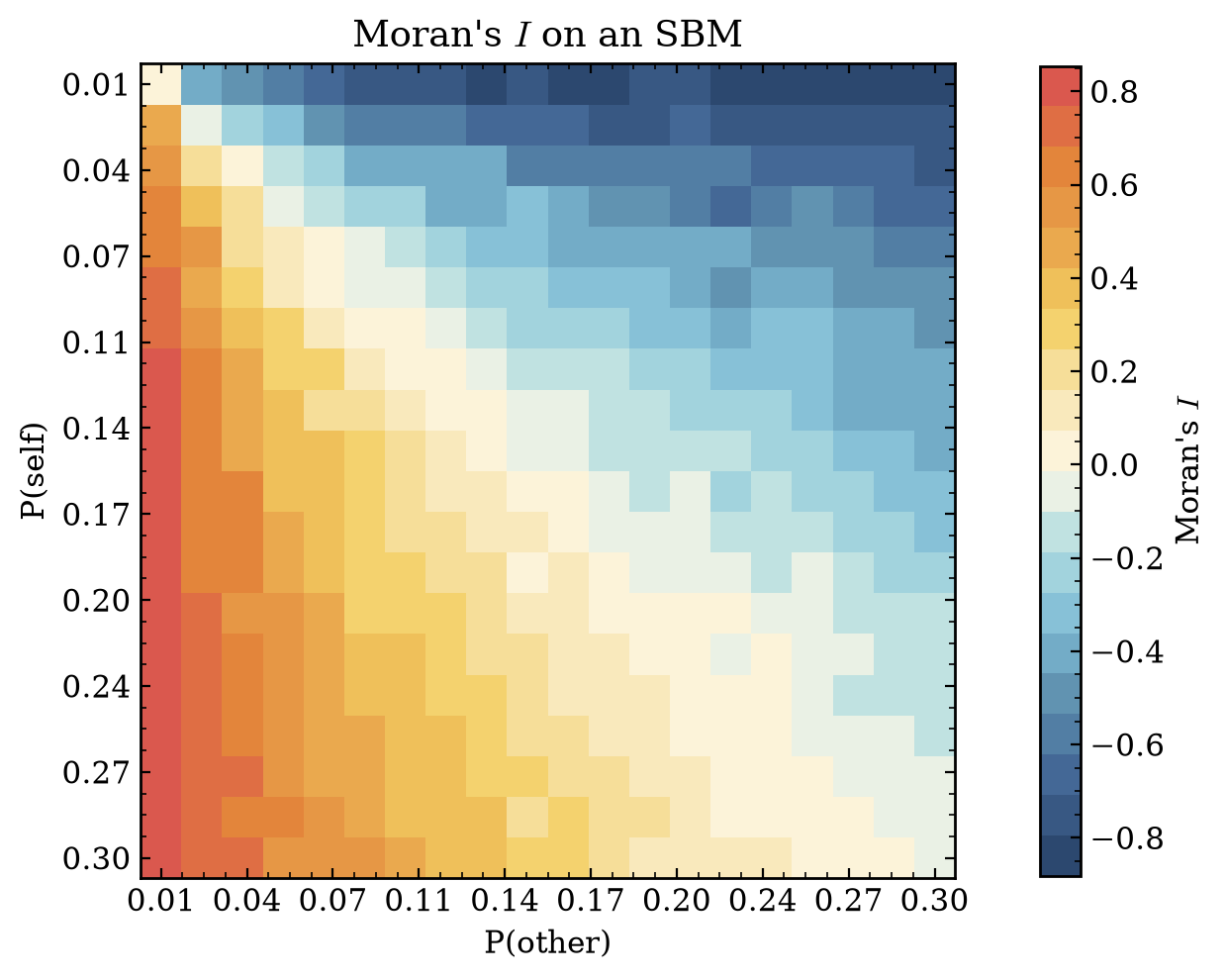
Basically we can use the metric directly with the above graph as
observed_statistic, expected_value,variance, z_score, p_value =  moran_i('attribute', g)
print(observed_statistic, p_value)
0.7673871040682526 1.4020007340385252e-92
results = np.zeros(shape = (20,20))

for index, ps in enumerate(np.linspace(0.01,0.3,20)):
  for index2, po in enumerate(np.linspace(0.01,0.3,20)):

    g = make_symmetric_sbm(ps, po, 2, 40, .6, -.6, .2 , .2, directed = True)
    observed_statistic, expected_value,variance, z_score, p_value =  moran_i('attribute', g)
    results[index, index2] = observed_statistic
fig, ax = plt.subplots(figsize=(6, 6))
im = ax.imshow(results, cmap=cmap)
norm = Normalize(vmin=results.min(), vmax=results.max())
sm = ScalarMappable(cmap=cmap, norm=norm)

cbar = fig.colorbar(sm, ax=ax, pad=0.08, shrink=.7)
cbar.set_label(r"Moran's $I$")
fig.tight_layout(pad=.5)

labels = [f"{i:.2f}" for i in np.linspace(0.01, 0.3, 10)]
ax.set_xticks(np.linspace(0, results.shape[1] - 1, 10))
ax.set_yticks(np.linspace(0, results.shape[0] - 1, 10))
ax.set_xticklabels(labels)
ax.set_yticklabels(labels)
ax.set_xlabel('P(other)')
ax.set_ylabel('P(self)')
ax.set_title("Moran's " + r"$I$" + " on an SBM")
plt.show()
Weighted Networks
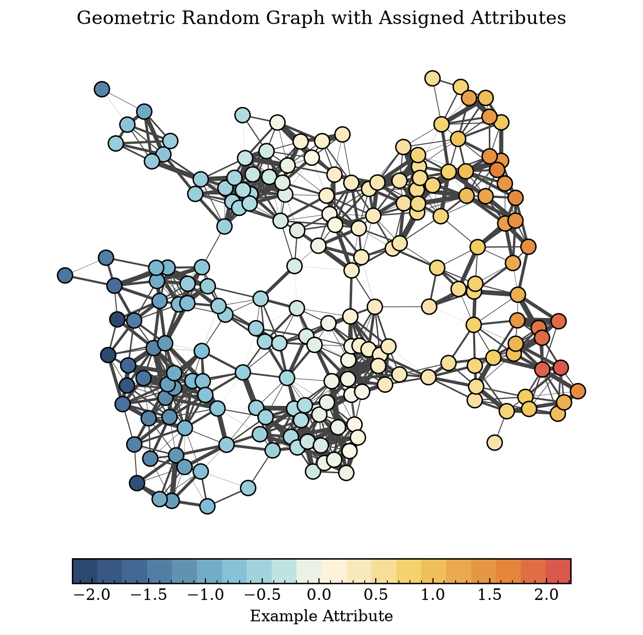
The metric also works on weighted networks and netseg implementation allows this. You have to supply a string that is embedded in the graph as an edge property.
g_grg = ig.Graph.GRG(200, 0.14, torus= False)
g_grg.vs['attribute'] = sorted(generator.standard_normal(g_grg.vcount()))
g_grg.es['weight'] = generator.standard_normal(g_grg.ecount())  * 1.6
fig, ax = plt.subplots(figsize = (8,8))

ig.plot(g_grg,
        layout = g_grg.layout_kamada_kawai(),
        vertex_color = get_custom_colors_hex(g_grg.vs['attribute']),
        edge_width = g_grg.es['weight'],
        target = ax)

cmap = ListedColormap(palette)
norm = Normalize(vmin=min(g_grg.vs['attribute']), vmax=max(g_grg.vs['attribute']))
sm = ScalarMappable(cmap=cmap, norm=norm)

cbar = fig.colorbar(sm, ax=ax, pad=0.01, orientation = "horizontal",
                    shrink = .8)
cbar.set_label('Example Attribute')
ax.set_title("Geometric Random Graph with Assigned Attributes")
plt.show()
observed_statistic, expected_value, variance, z_score, p_value = moran_i('attribute', g_grg, weights = 'weight')
print(observed_statistic, p_value)
1.8010364174973448 0.12734551907963637
Null Models and Significance
Moran’s \(I\) on its own is just a number. A value of \(0.4\) means little until we know what \(I\) would look like if there were no spatial structure at all. That is what the rest of the returned values are for. The function hands back five things in order, the observed statistic, the expected value under the null, the variance under the null, the z score, and the p-value.
The observed statistic is \(I\) computed on the real attribute as it sits on the graph. Everything after it tells you whether that number means anything. The expected value is where \(I\) would sit with no spatial signal, and on a structureless graph that is not zero but a small negative offset \(-1 / (n - 1)\). The variance is how much \(I\) wobbles around that expectation by chance. The z score puts the observed value on that scale, how many standard deviations the real \(I\) sits from the null expectation, so a large positive z score is strong positive autocorrelation and a value near zero is a field the null would produce without trouble. The p-value is the two-sided tail, the chance of seeing an \(I\) at least as far from the expectation as the observed one when there is no real structure. A small p-value means the null almost never reaches our \(I\) and we read the pattern as real. A large one means random arrangements land there often, so a high \(|I|\) on its own is not evidence of anything.
The function builds that null two ways. With no null models it uses the closed form, the expectation \(-1/(n-1)\), the randomization variance, and a p-value from the normal approximation. This is fast and needs no extra graphs, and it is the right default when the normal approximation holds. When the user passes a list of null models it drops the closed form and reads the null off those graphs instead. It holds the attribute fixed, recomputes \(I\) on each null model, and takes the expected value as their mean, the variance as their sample variance, and the p-value as the empirical two-sided tail. This is what the custom null buys. The closed form assumes one kind of randomness, values shuffled freely across a fixed graph. A custom null lets the user encode a different notion of structureless, a family of degree-preserving rewirings or any set of graphs sharing a property worth controlling for. The question shifts from whether the pattern beats free reshuffling to whether it beats the null family the user built. The attribute stays pinned to the same node ordering across every null model, so each null model must match the observed graph in node count and ordering, otherwise the function raises.
References
Cressie, N. (2015). Statistics for spatial data. John Wiley & Sons.
Duchin, M., Murphy, J. M., & Weighill, T. (2023). Measuring segregation via analysis on graphs. SIAM Journal on Matrix Analysis and Applications, 44(1), 80-105.
Moran, P. A. P. (1950). “Notes on Continuous Stochastic Phenomena”. Biometrika. 37 (1): 17–23. doi:10.2307/2332142. JSTOR 2332142. PMID 15420245.
Ising, E. Beitrag zur Theorie des Ferromagnetismus. Z. Physik 31, 253–258 (1925). (In German)